Lab 1.2 “Hello World!” QGIS Bootcamp
- Adding spatial data
- Exploring spatial data attributes
- Adding a field
- Symbolizing our map
- Filtering our fields
- Saving Our Map Layer for Web Mapping
- Adding non-spatial data
- Lab Questions
Adding spatial data
Important: Before starting this lab, you must have completed the pre-lab and part 1. This means you should have already installed QGIS and a local copy the lab.
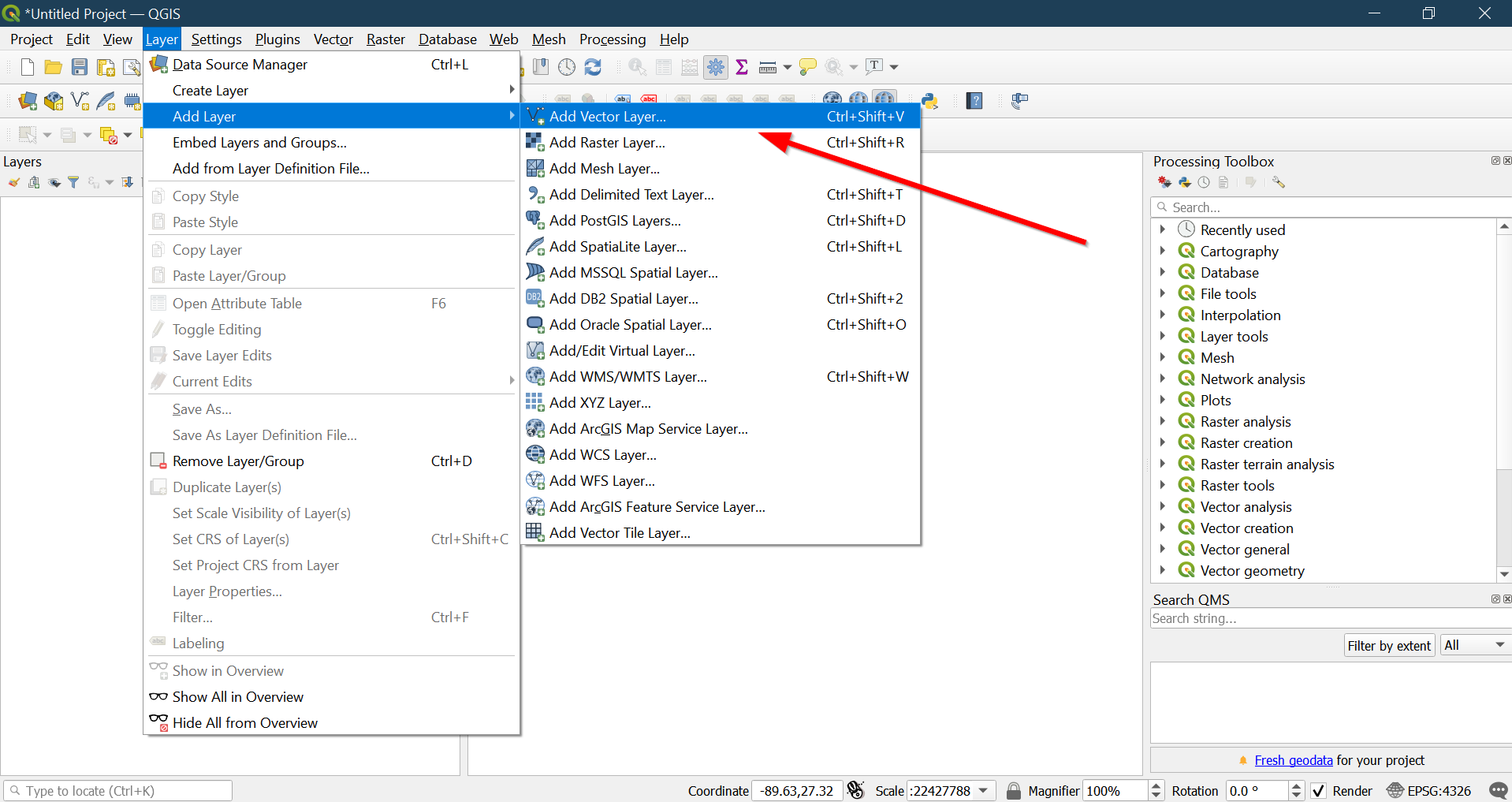
- Click on
Layer
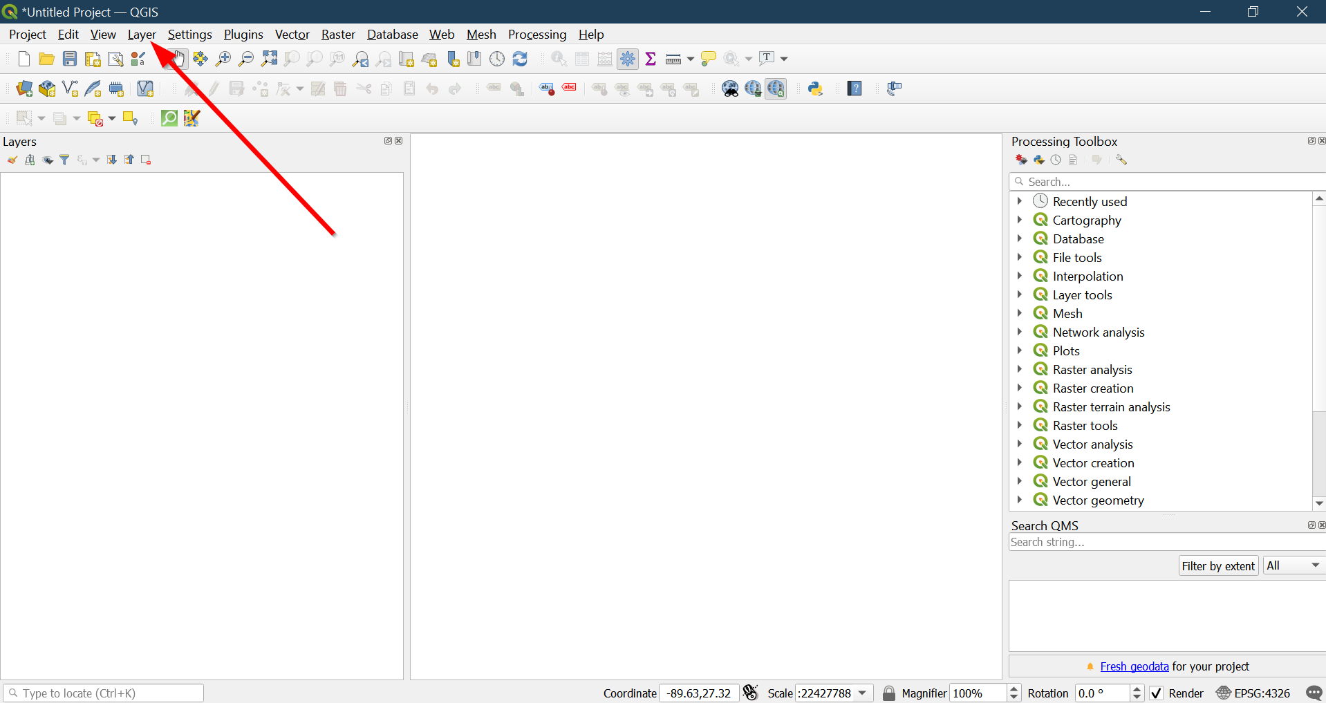
Add LayerAdd vector layer
- Locate the file
**CA_Counties.shp**
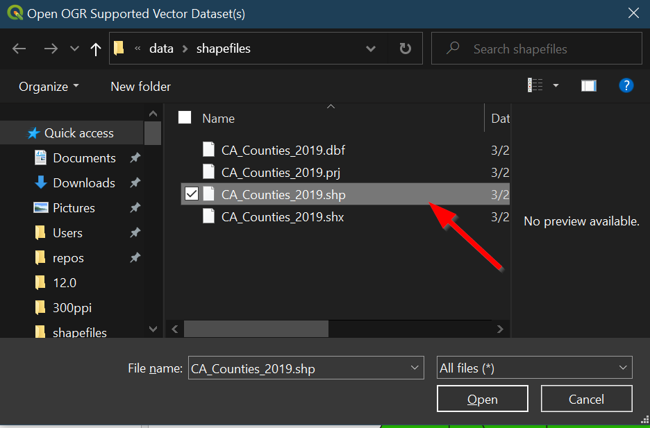
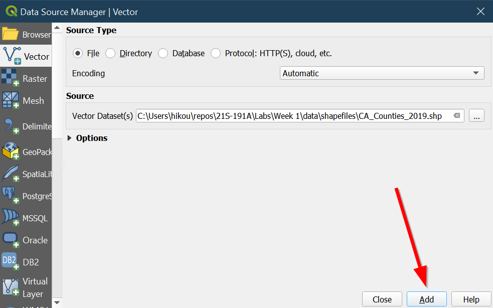
- Click
Addto add it to your QGIS project.
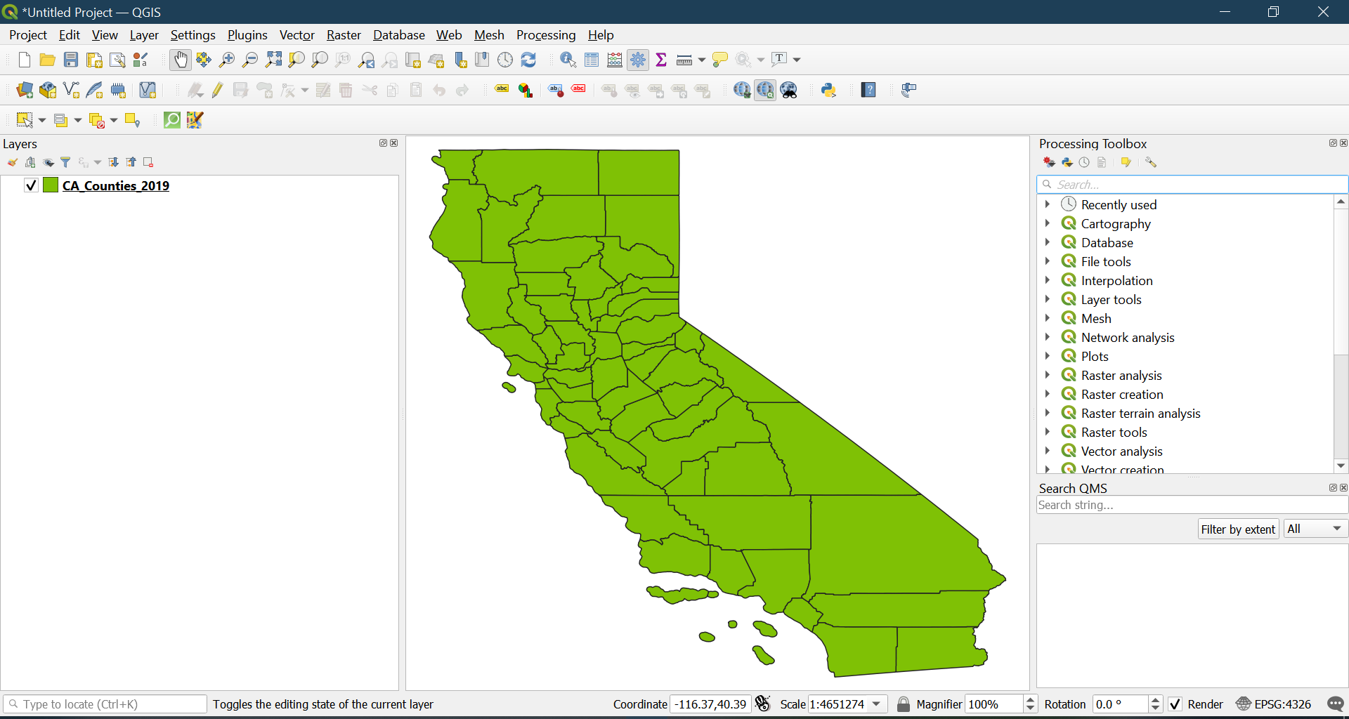
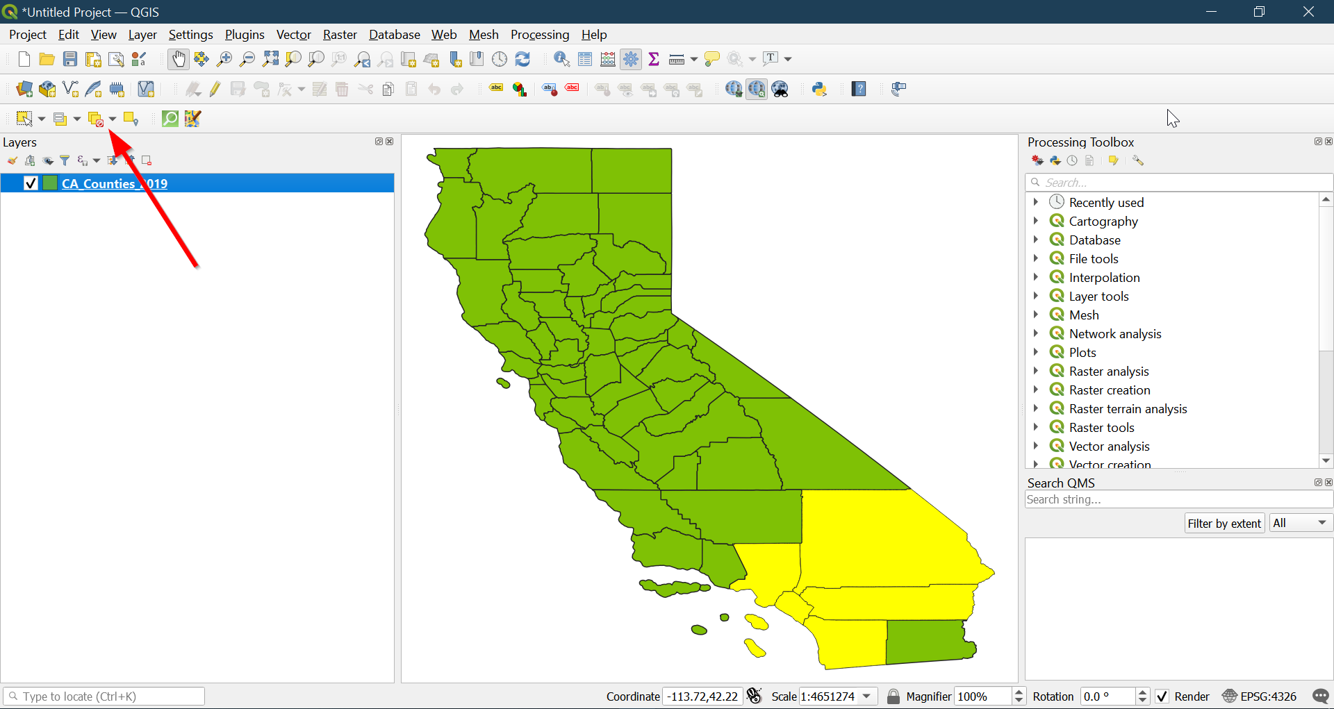
- Counties in California should now appear:
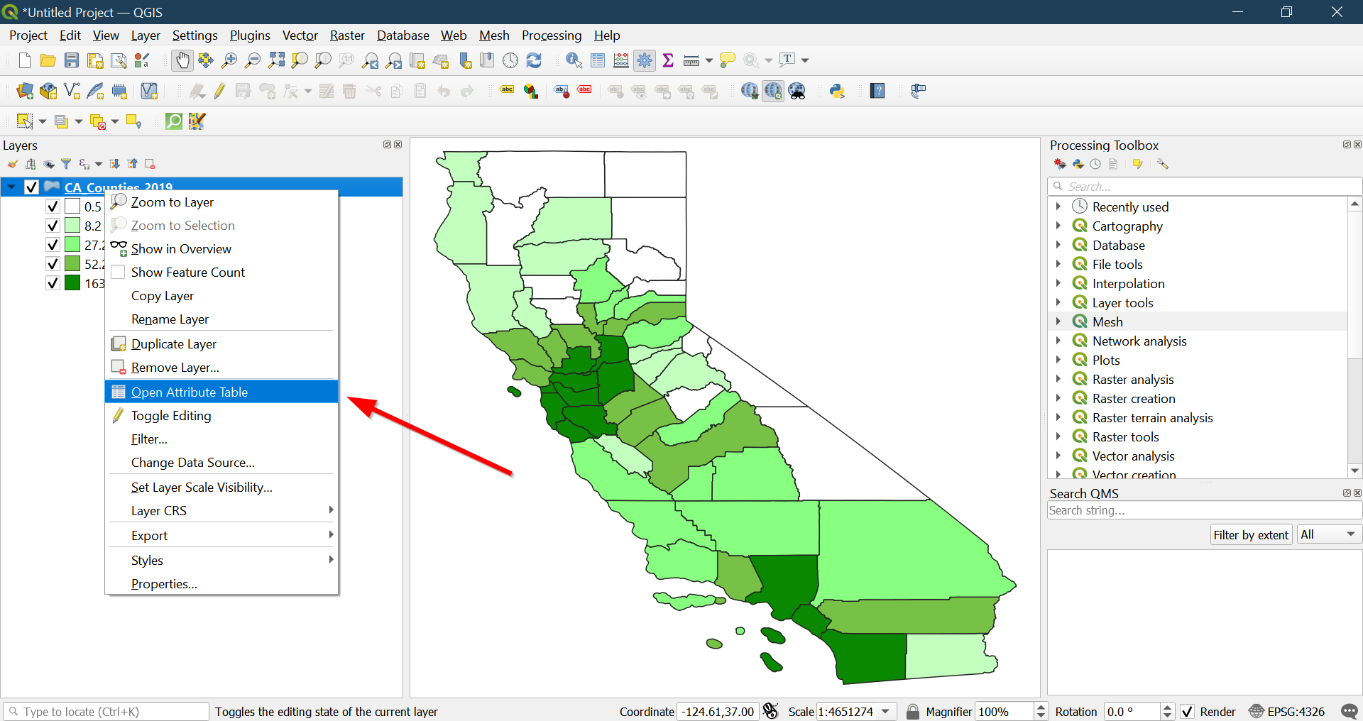
Exploring spatial data attributes
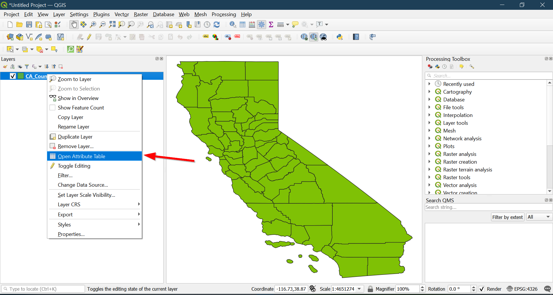
- In the
Layerspanel, right click on the layer**CA_Counties_TIGER2016**
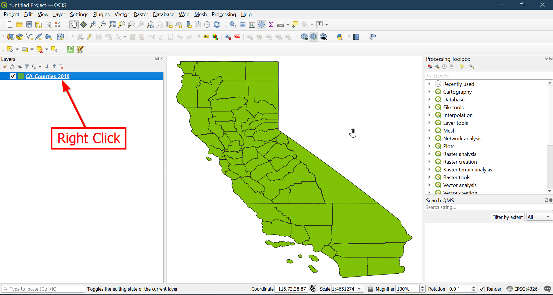
- Click on
Open Attribute Table
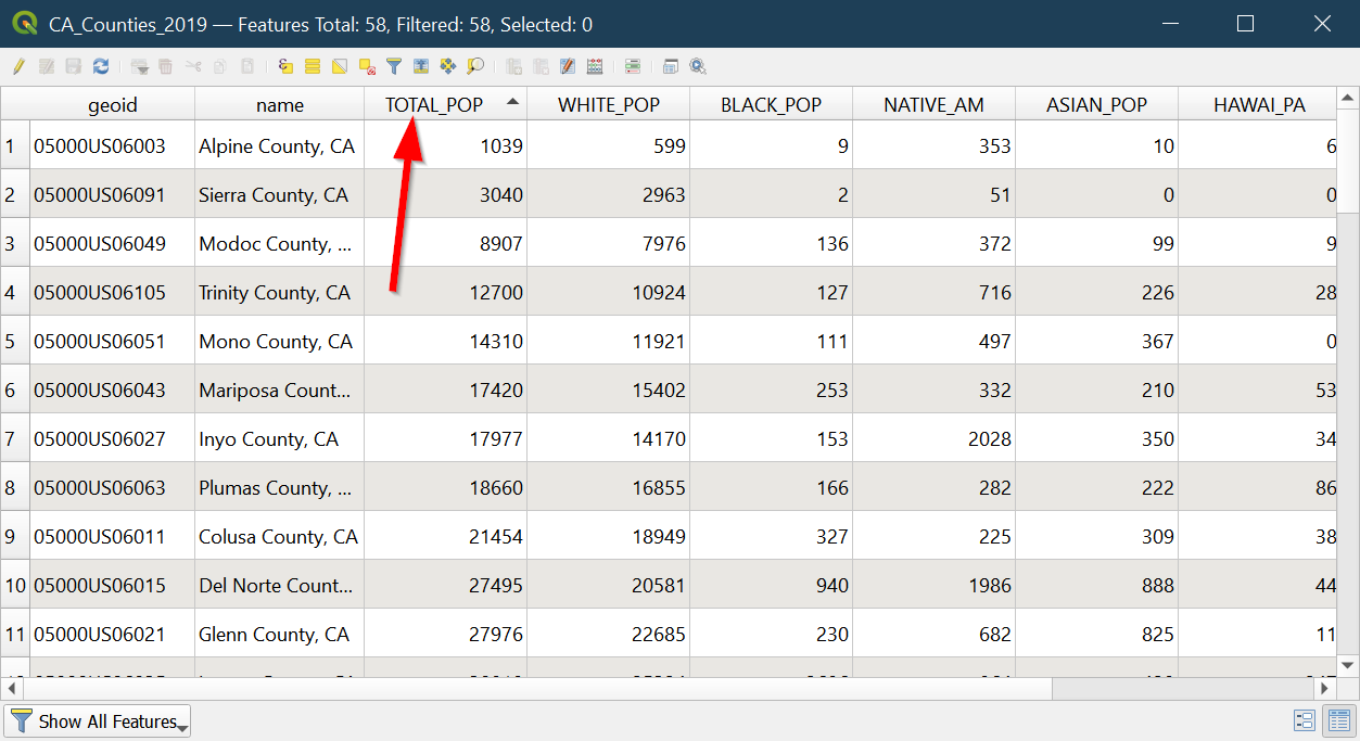
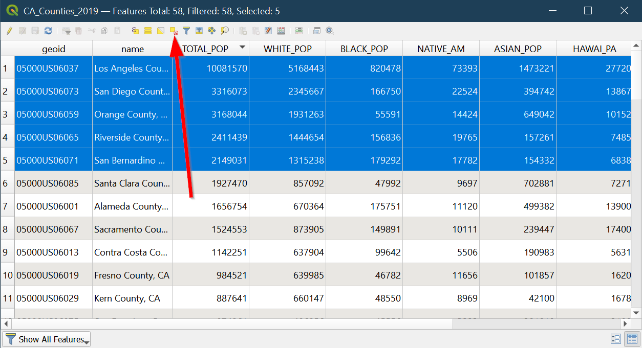
- Now you can see the attributes of each of the spatial data shown in the map:
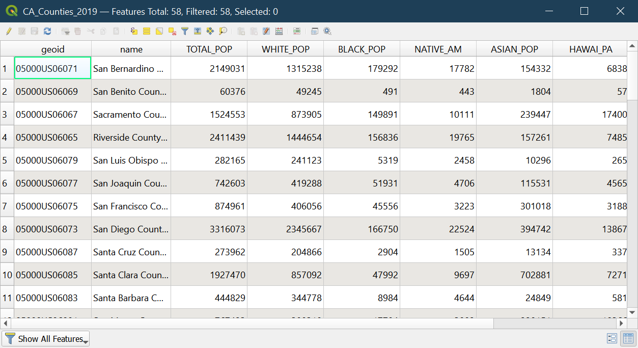
- You can click on the headers to sort, so let’s find the most populous county in California by scrolling to
**TOTAL_POP**and clicking on it:
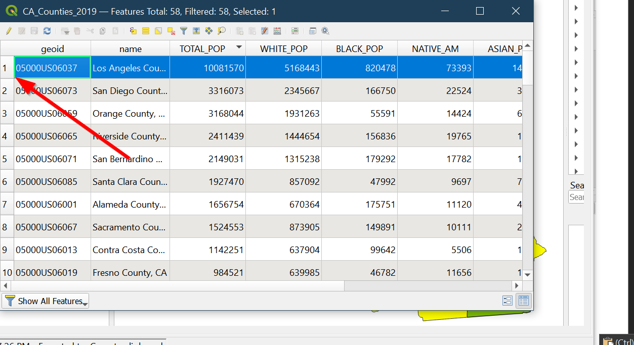
- We can highlight the county by click on the number box with the number 1 next to it:
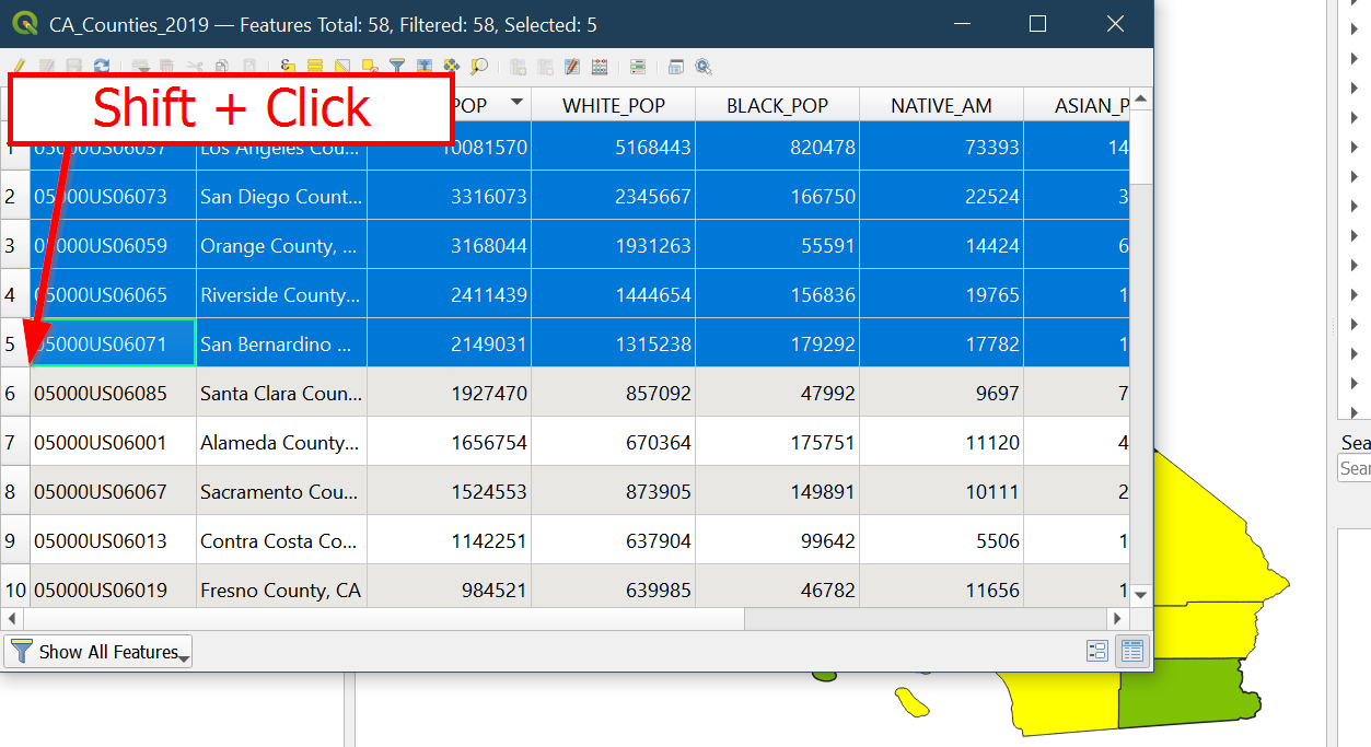
Note: Shift + Click down to select multiple rows:
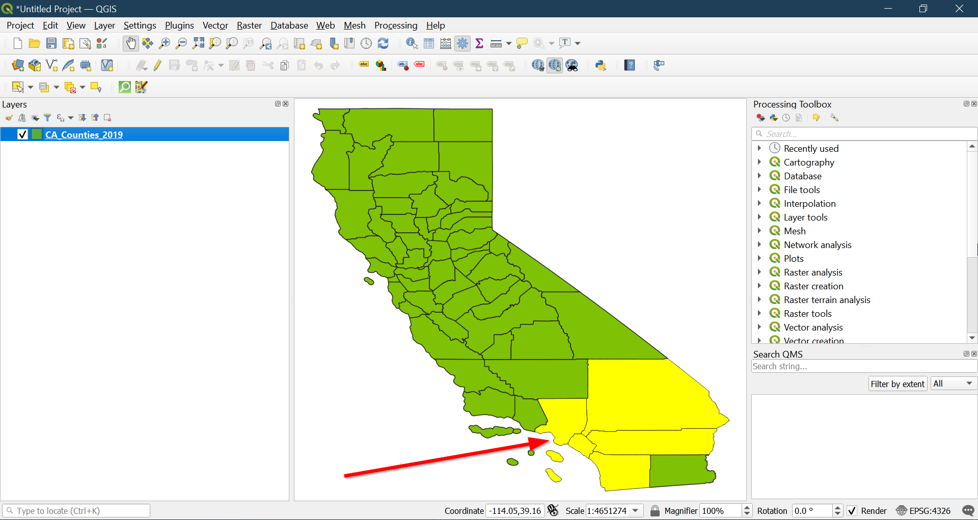
- Return to the map to see the most populated counties according to the American Community Survey 2019 data in California highlighted:
-
Clear your selection in the following ways:
- Clicking the deselect button in the general interface:
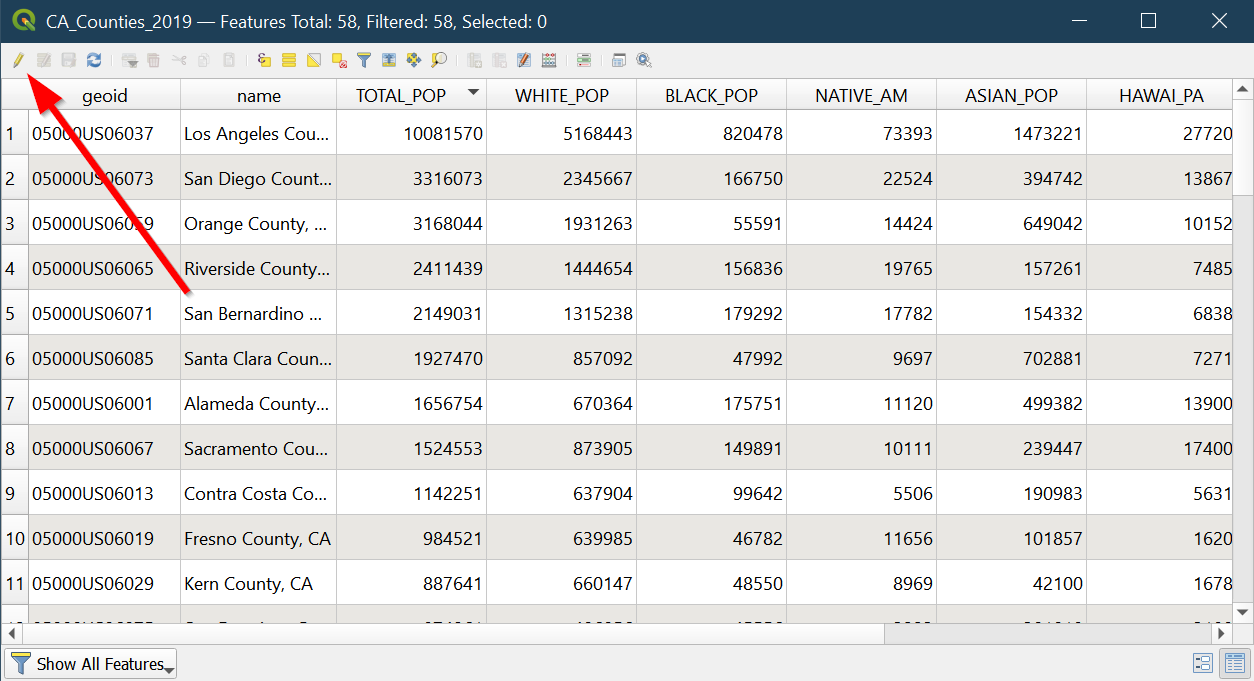
- Or the deselect button in the attribute table:
Adding a field
Since bigger areas are most likely to have more people, we need to factor that in to see where most people in the state are likely to be found. We will do a population density calculation, which is simply
number of people divided by total area.
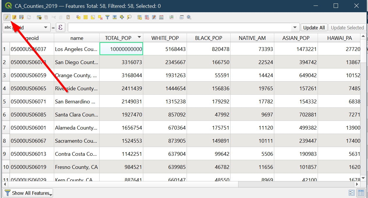
- Click the
edittool to enable making changes:
- Warning! When you are in
editormode you can click on any cell to directly edit it:
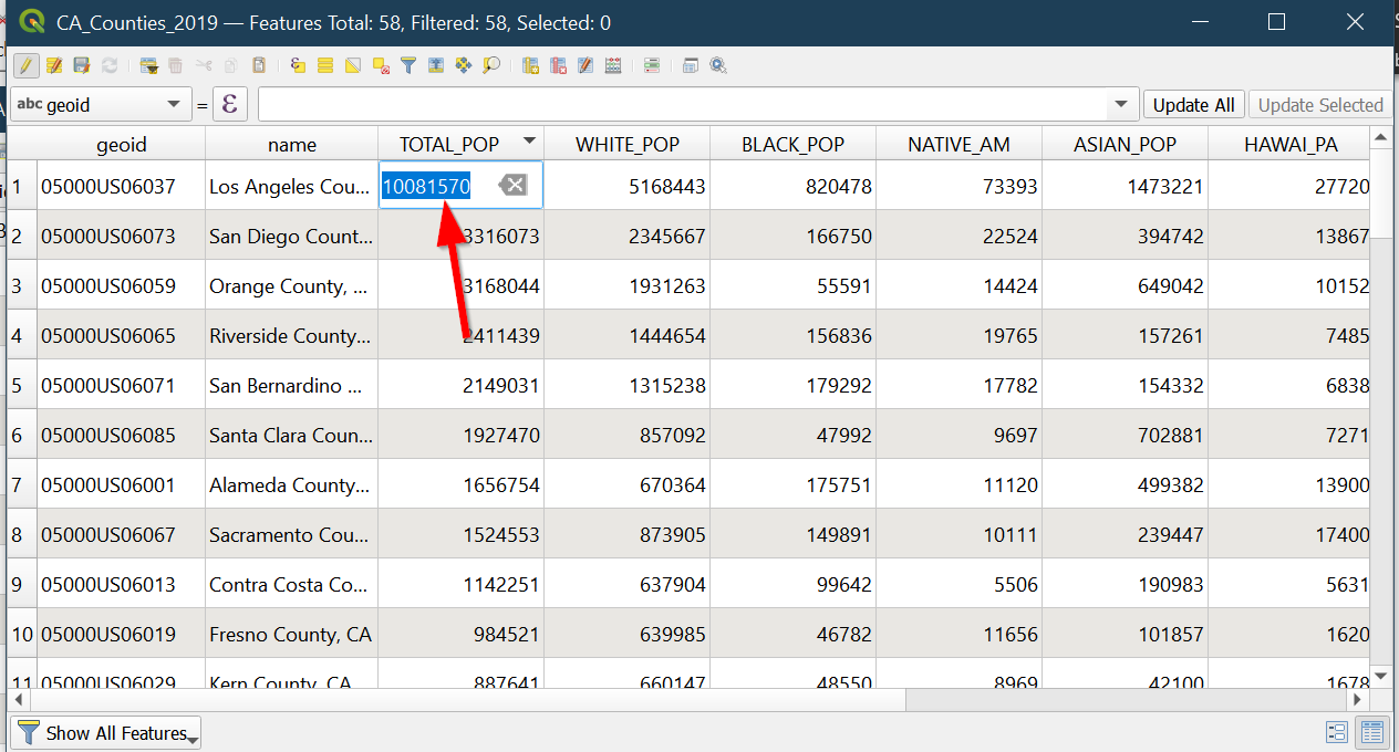
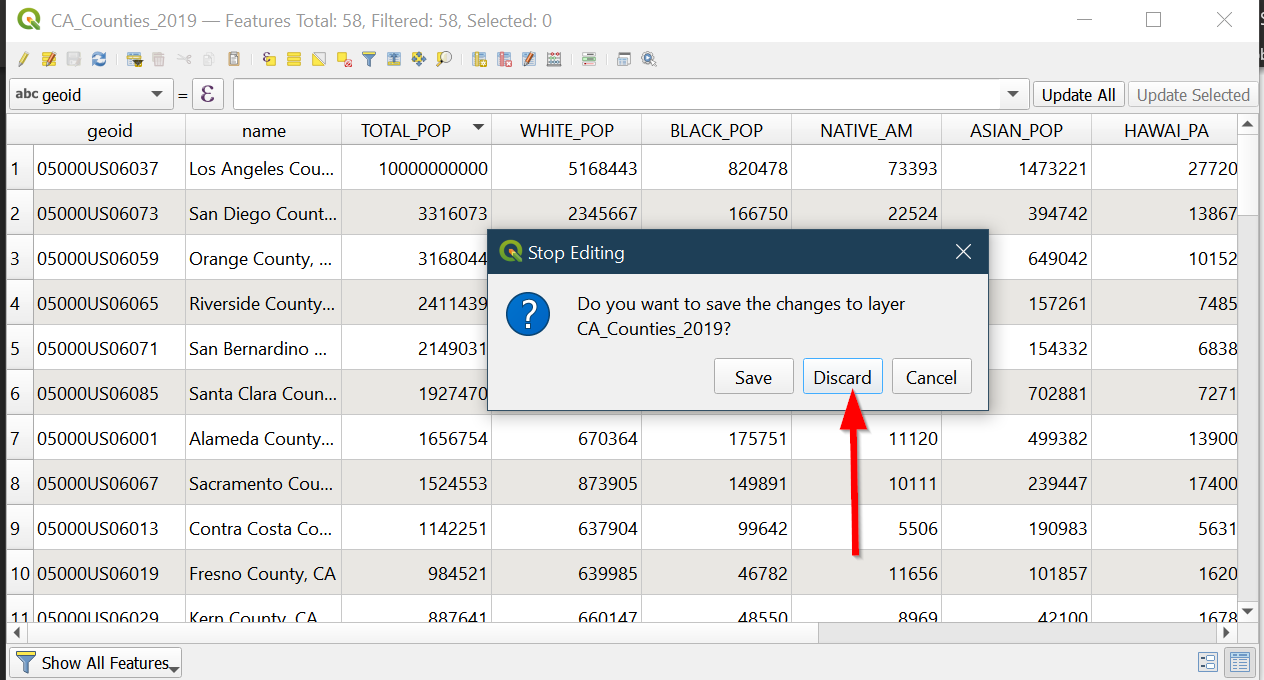
-
If you accidentally made edits, turn off editing mode by clicking the pencil again:
-
Choose
Discard:
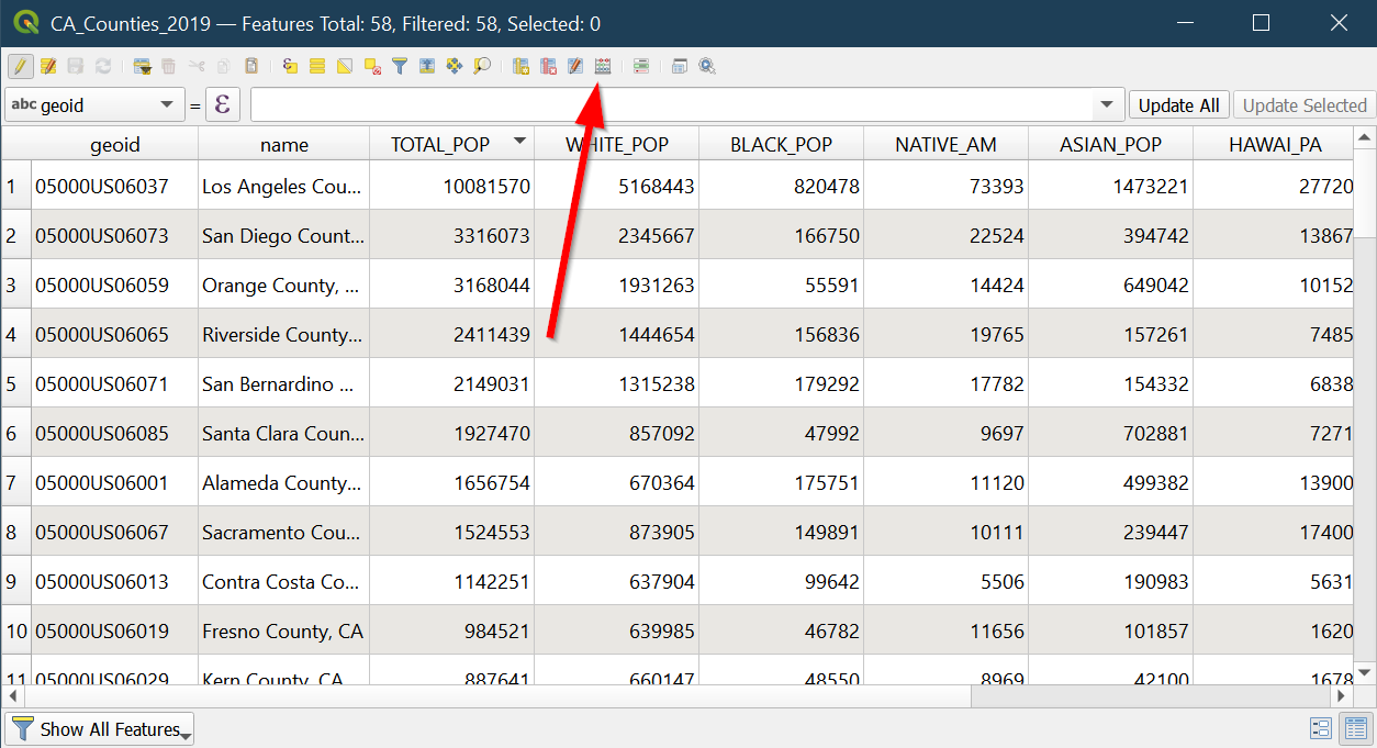
- Next click the
Field Calculatorbutton:
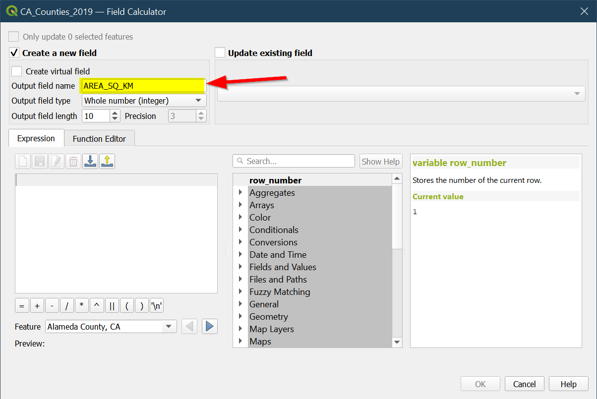
- The field calculator window will appear:
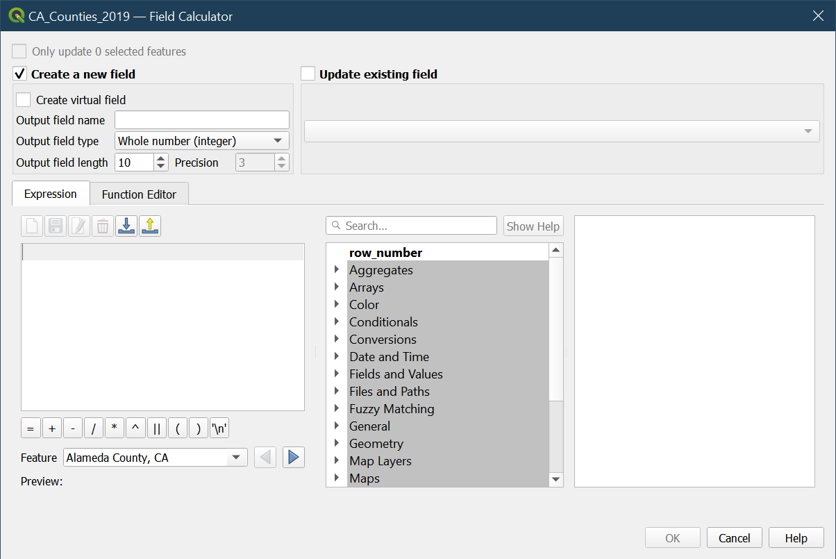
- Click on
Output field nameand type inAREA_SQ_KMwhich will beArea in square kilometers.
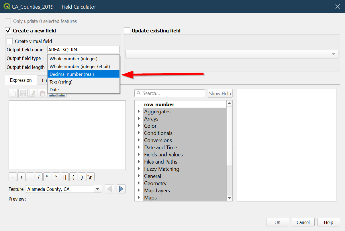
- Click on field type and choose
Decimal Number (real)
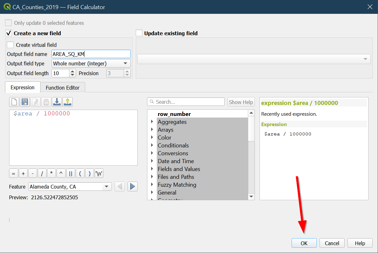
- In the Expression box type in the following:
$area / 1000000
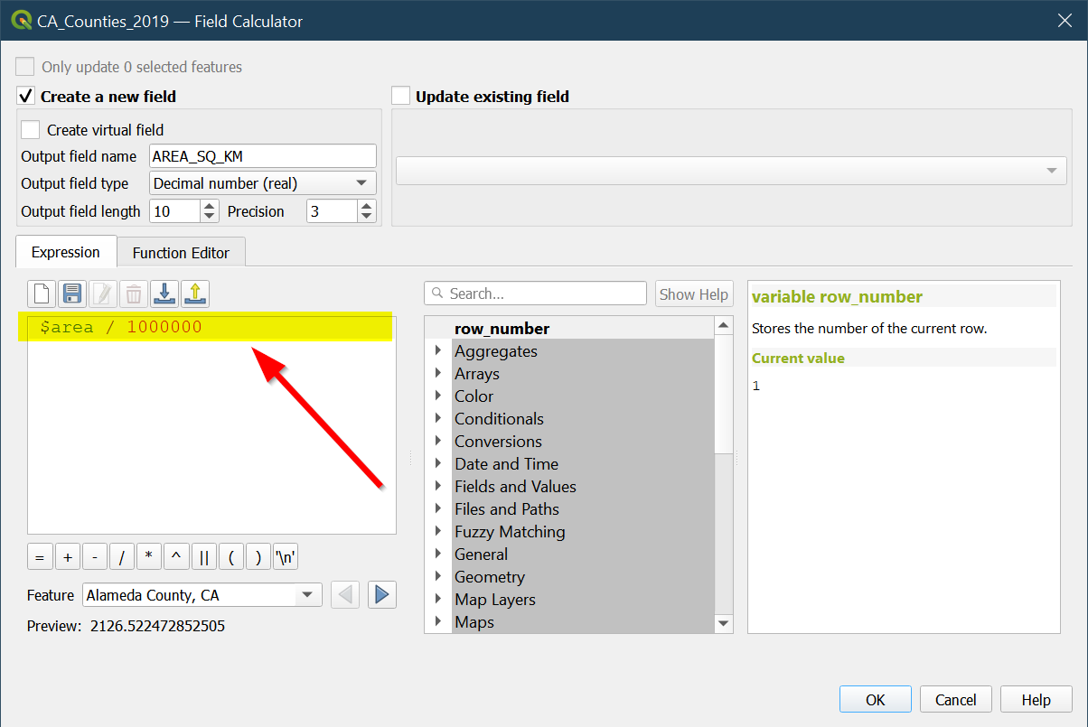
- If correctly done, you can see the preview will show the value:
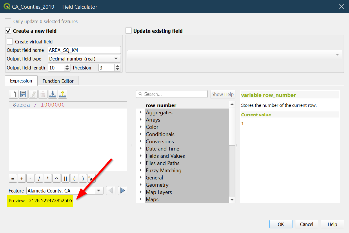
- Click
OK:
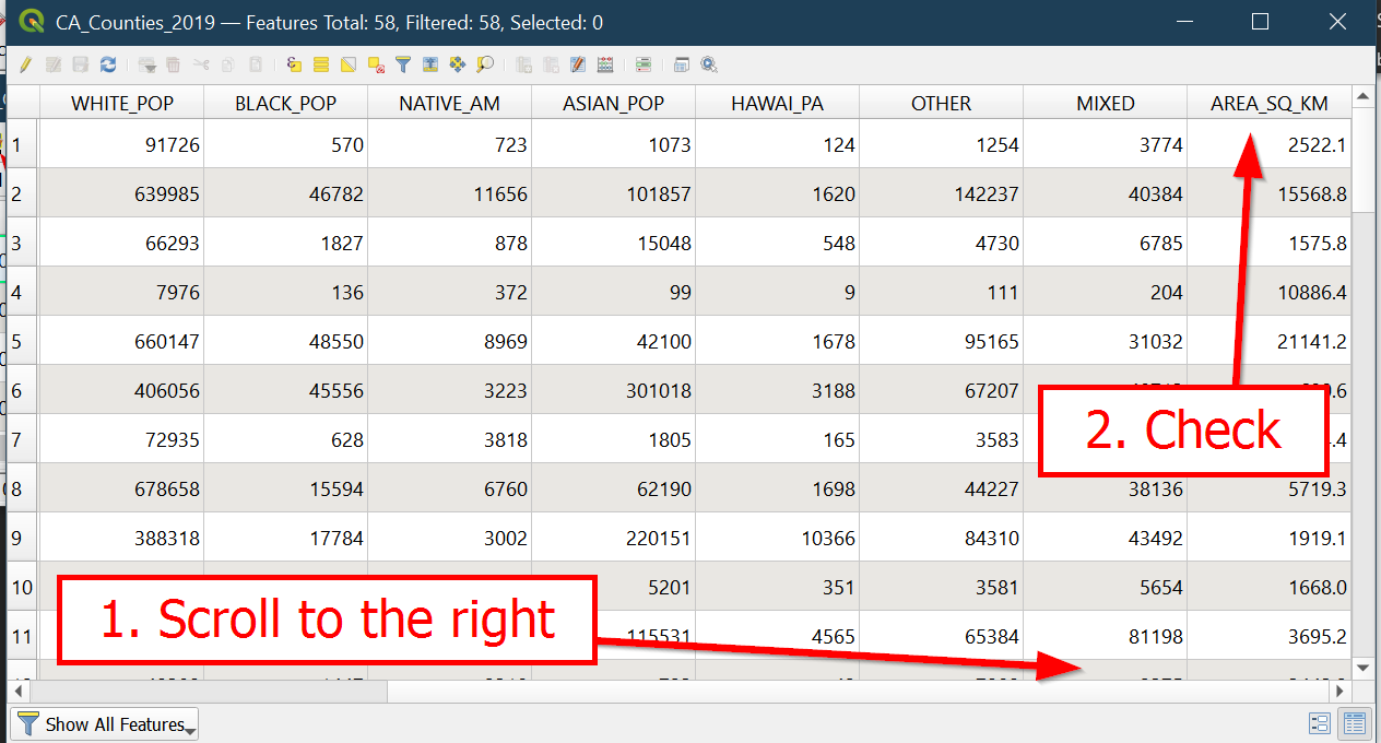
- You can see our new field all the way on the right side:
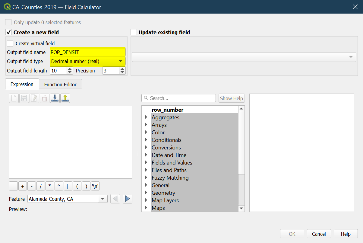
- Open the
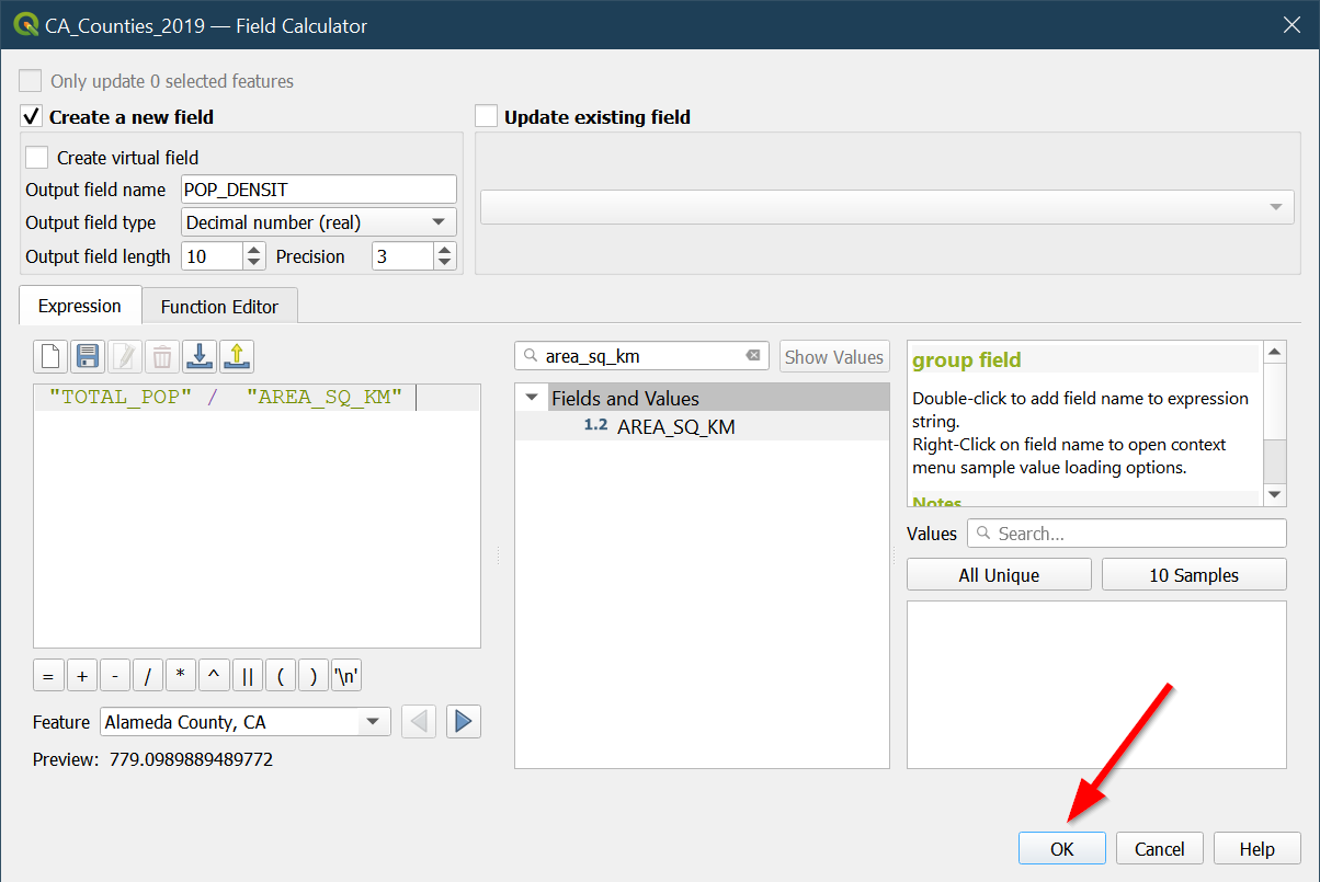
Field Calculatoragain and create a new field calledPOP_DENSITwithDecimal number (real):
- Locate the search box, this place is helpful for creating expressions.
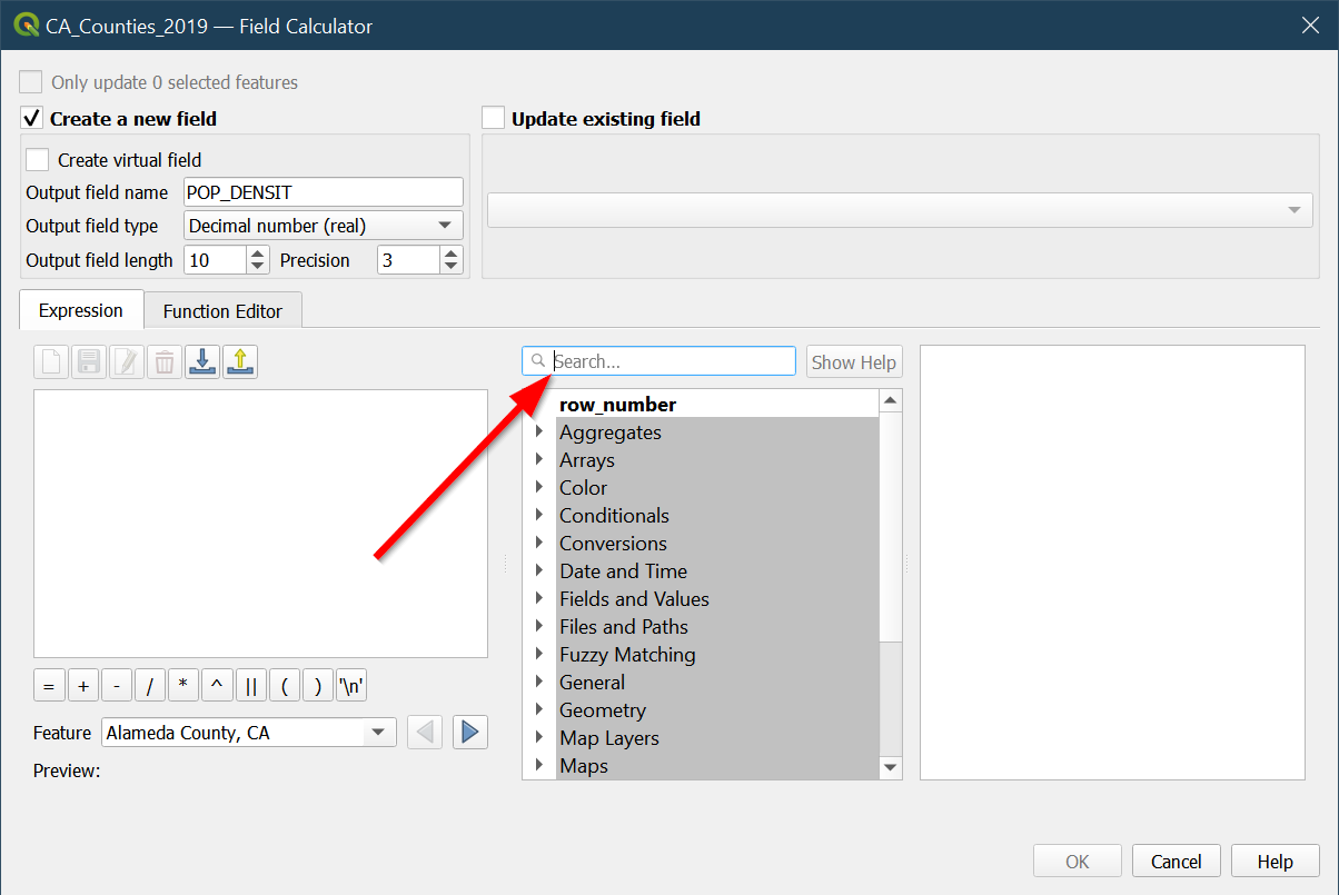
- In the search box type in
total_popand double click on the result:
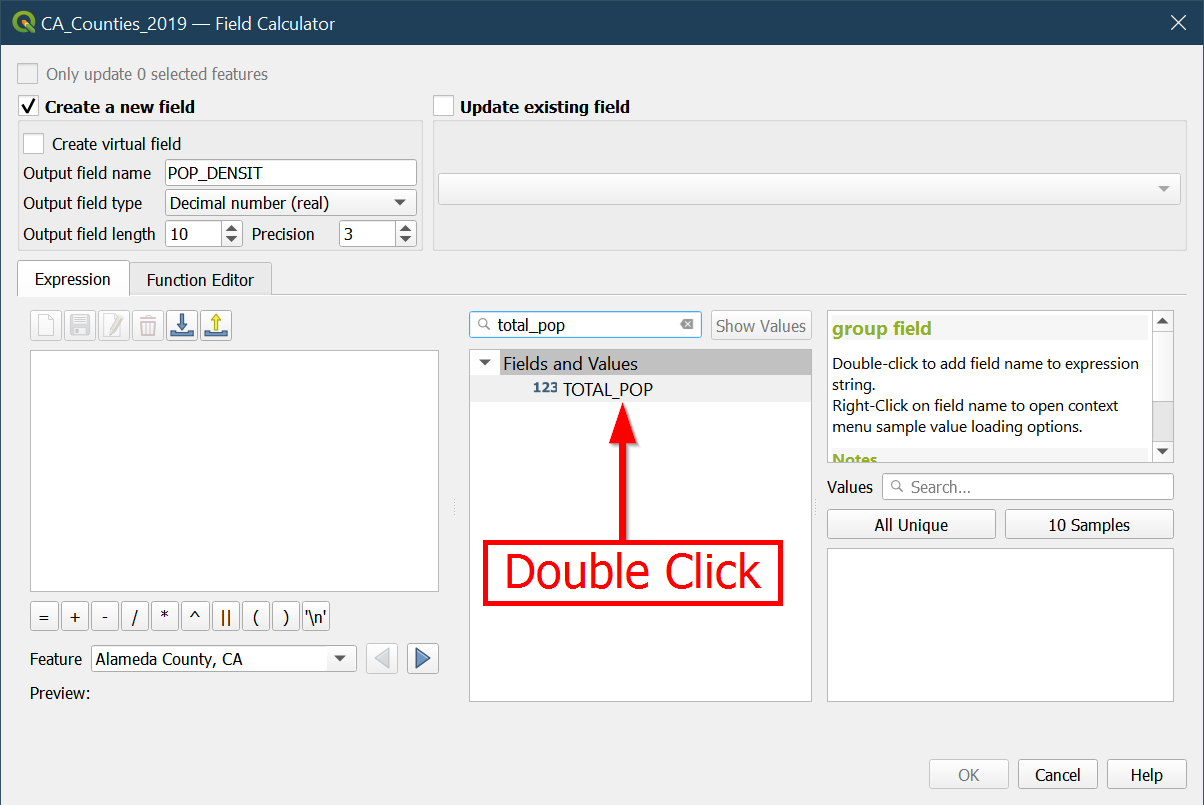
- Note: The help on the right side explains more detail about what is being selected in the search box.
-
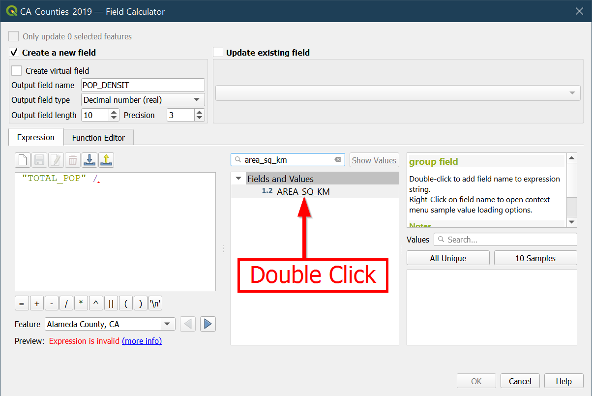
Add a
/for divide -
Search for
area_sq_kmand add it to our expression:
- The final expression should be:
"TOTAL_POP" / "AREA_SQ_KM"
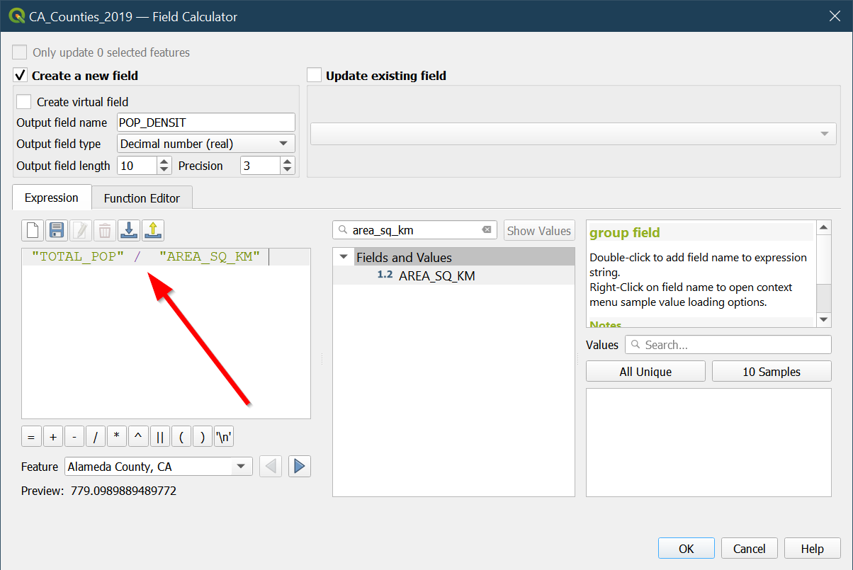
- Check the preview:
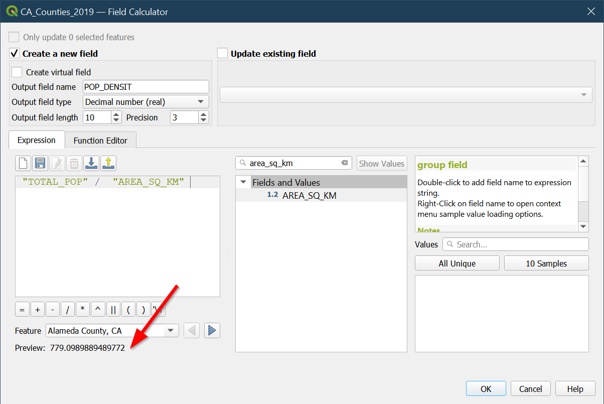
- Hit OK:
- Check to see if the
POP \ DENSITcolumn is there:
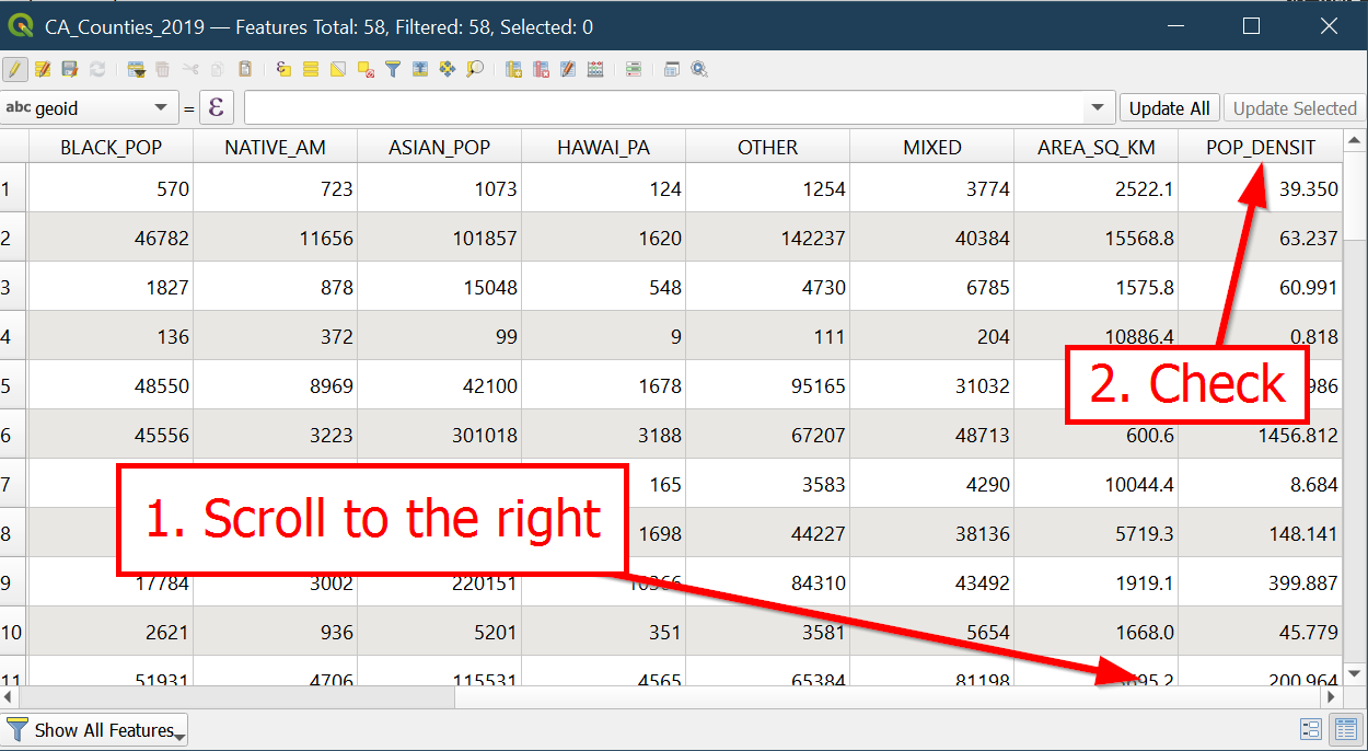
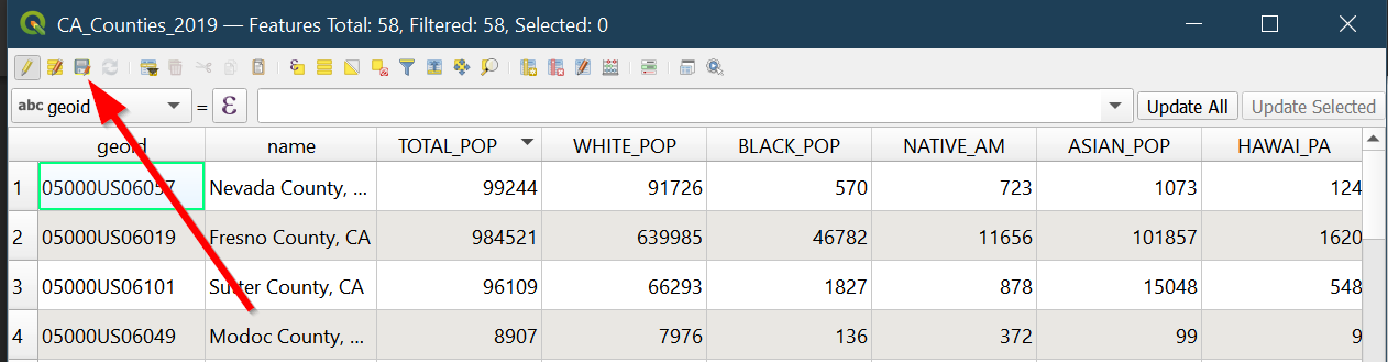
- If you have successfully calculated the population density for all
the counties in California, then click the
savebutton to save our edits:
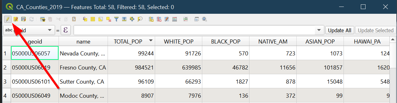
- Turn off the editing tool as we are done with it:
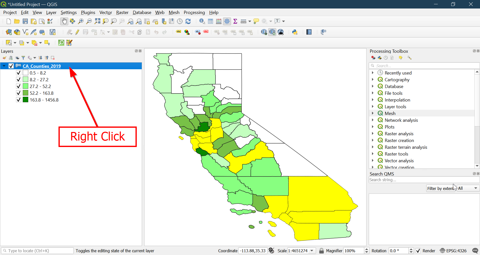
Symbolizing our map
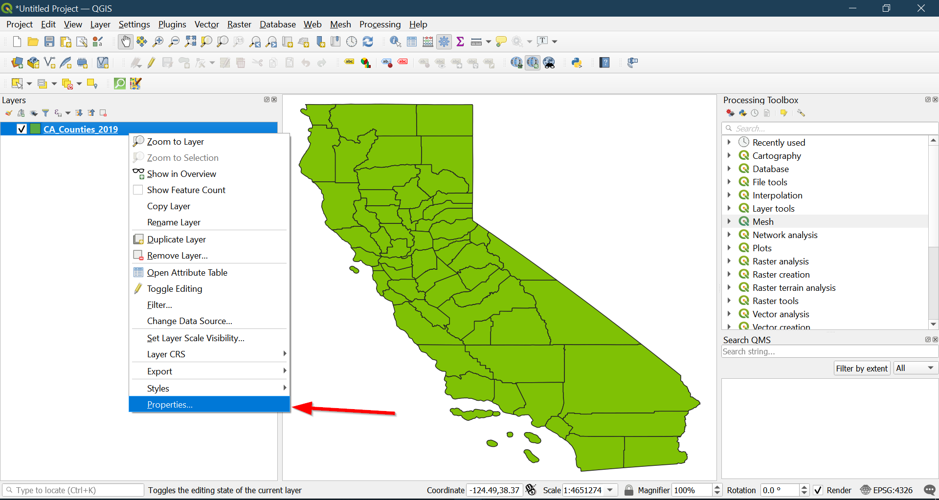
- Right click on our layer and go to
Properties:
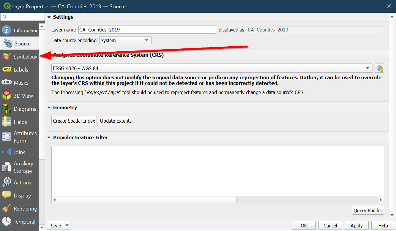
- Click on
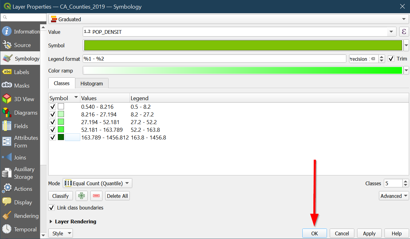
Symbology:
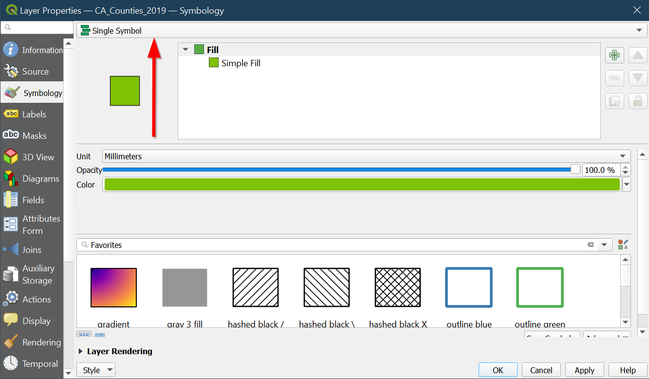
- From there, click on
Single Symbolto change which data fields are being used for map creation:
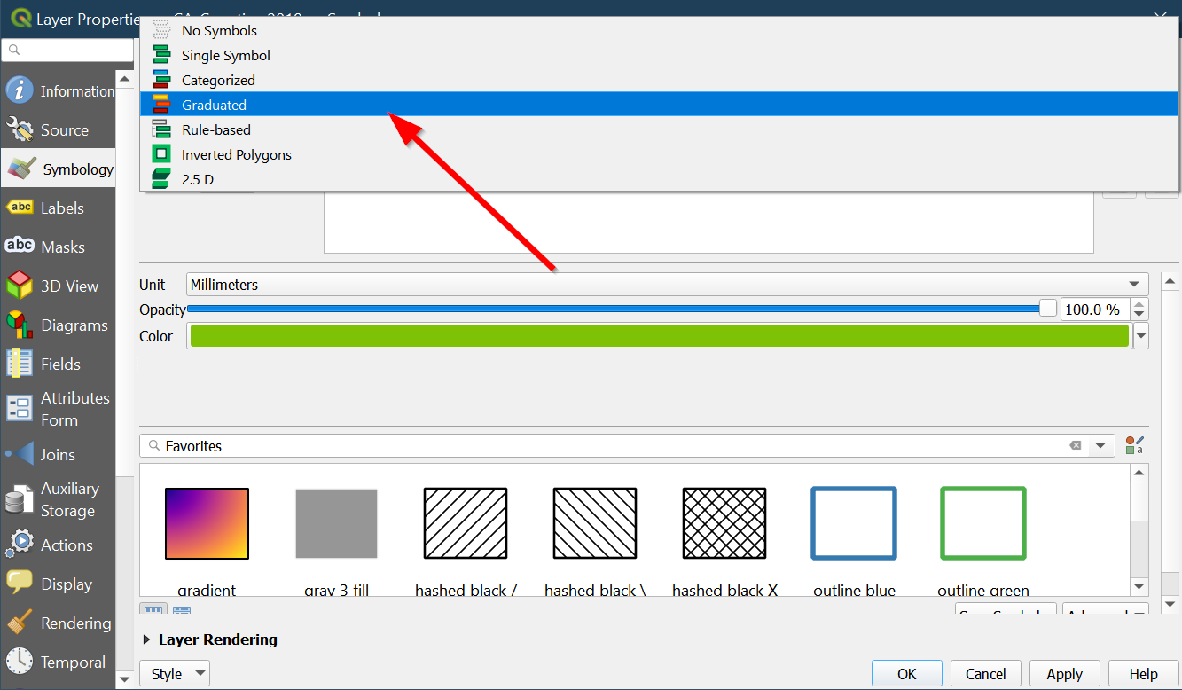
- If we were working with qualitative data fields then we would use
categorized, however we are going to be looking at our population density data field, so we should usegraduated:
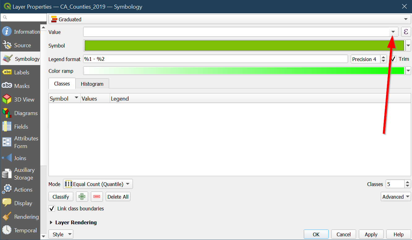
- Click the dropdown arrow near
Valueto see the list of fields:
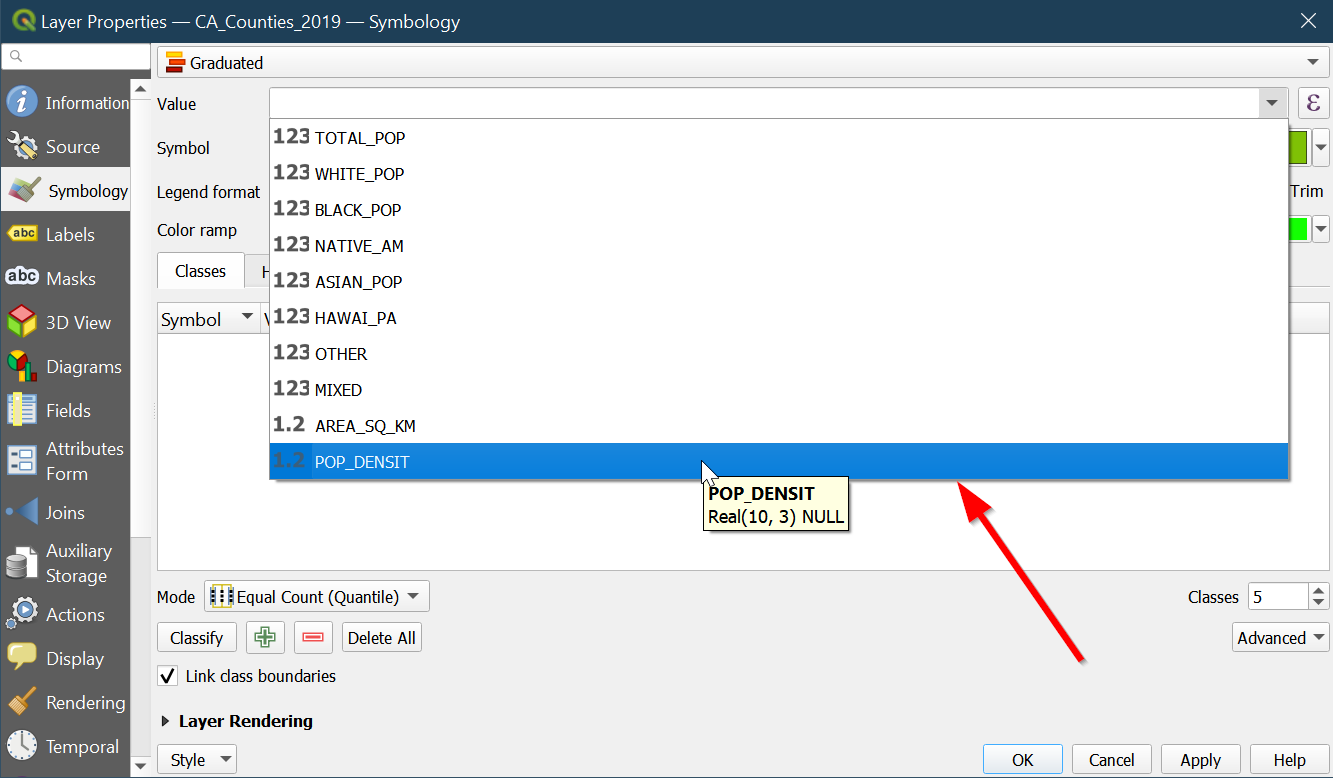
- Choose
POP_DENSIT:
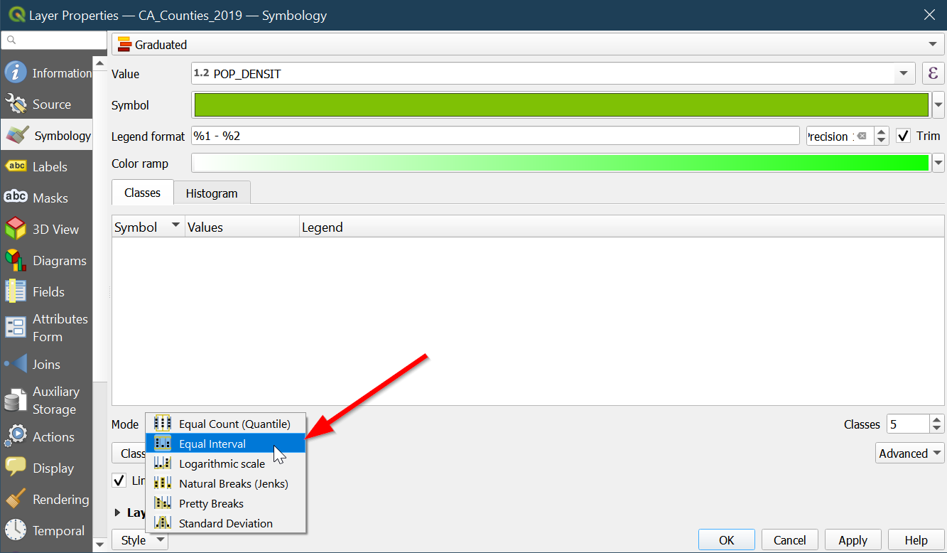
- Change the
ModetoEqual Intervalwhich means that the breaks between values are evenly spaced apart (i.e. 0-5, 5-10,10-15):
- You can click histogram to get a better sense of the data and which statistical mode you should use (but since this is not a stats class, I won’t spend much more time on this):
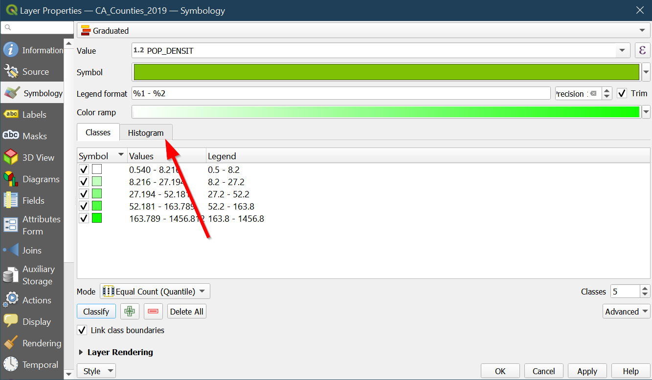
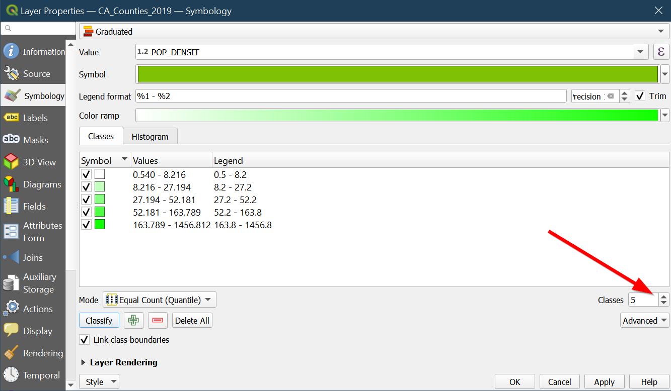
- You can also change the number of
classes(or breaks) by clicking here:
-
Click
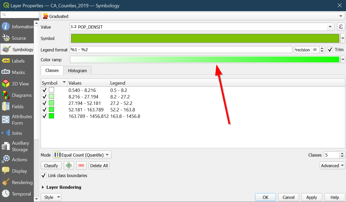
OKto apply our changes to the map: -
You can change the colors by clicking on
Color ramp:
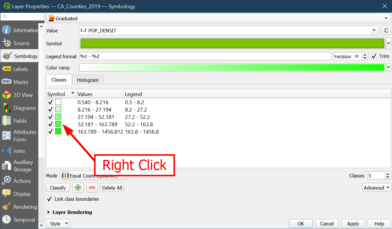
- Or individually by right clicking the square colored boxes:
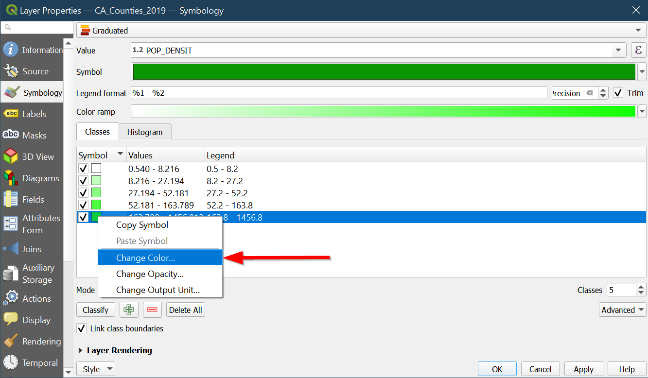
- Choose
change colorand adjust the color wheel:
- When satisfied with your changes click
OKto close the dialogue box:
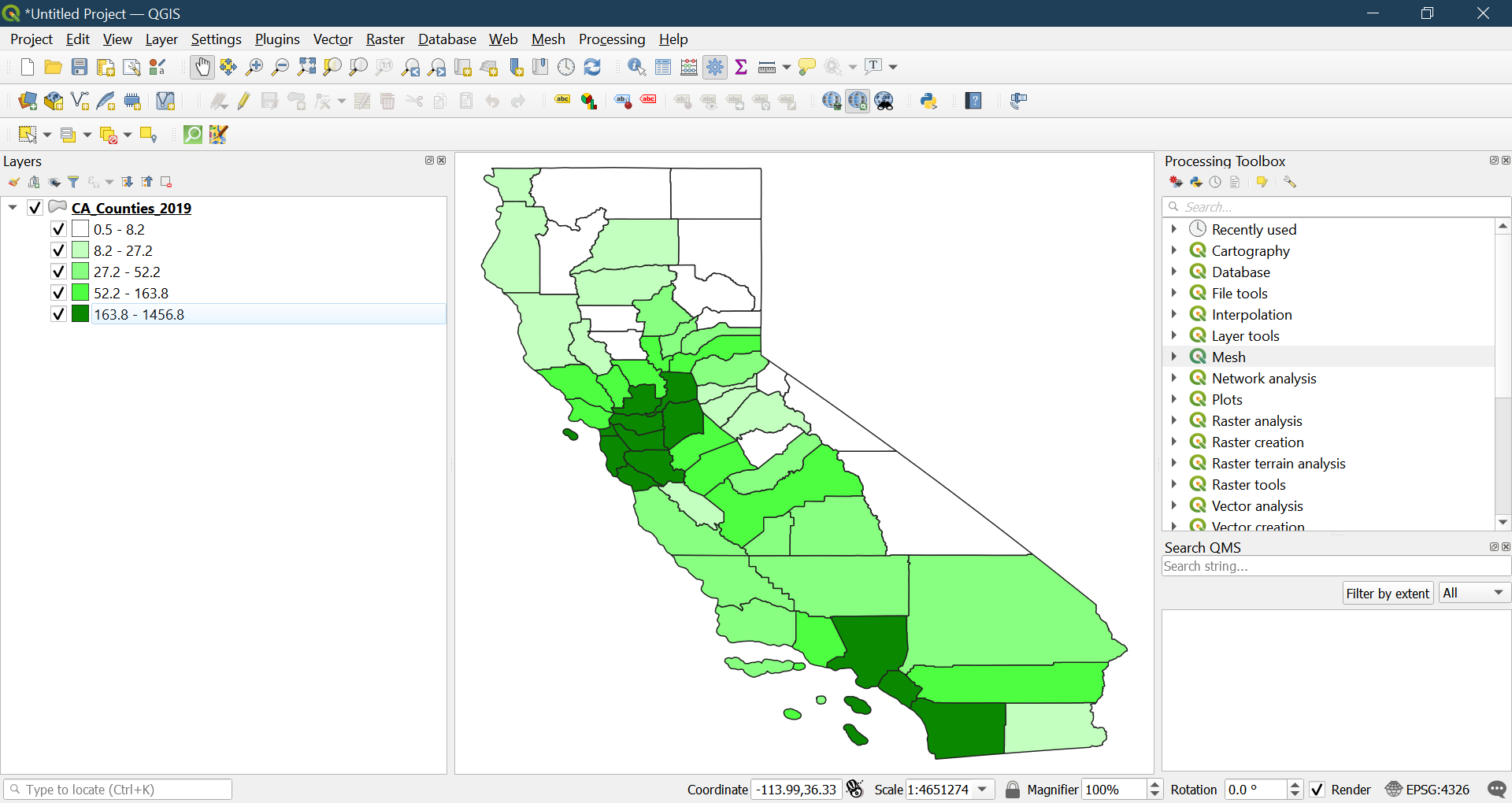
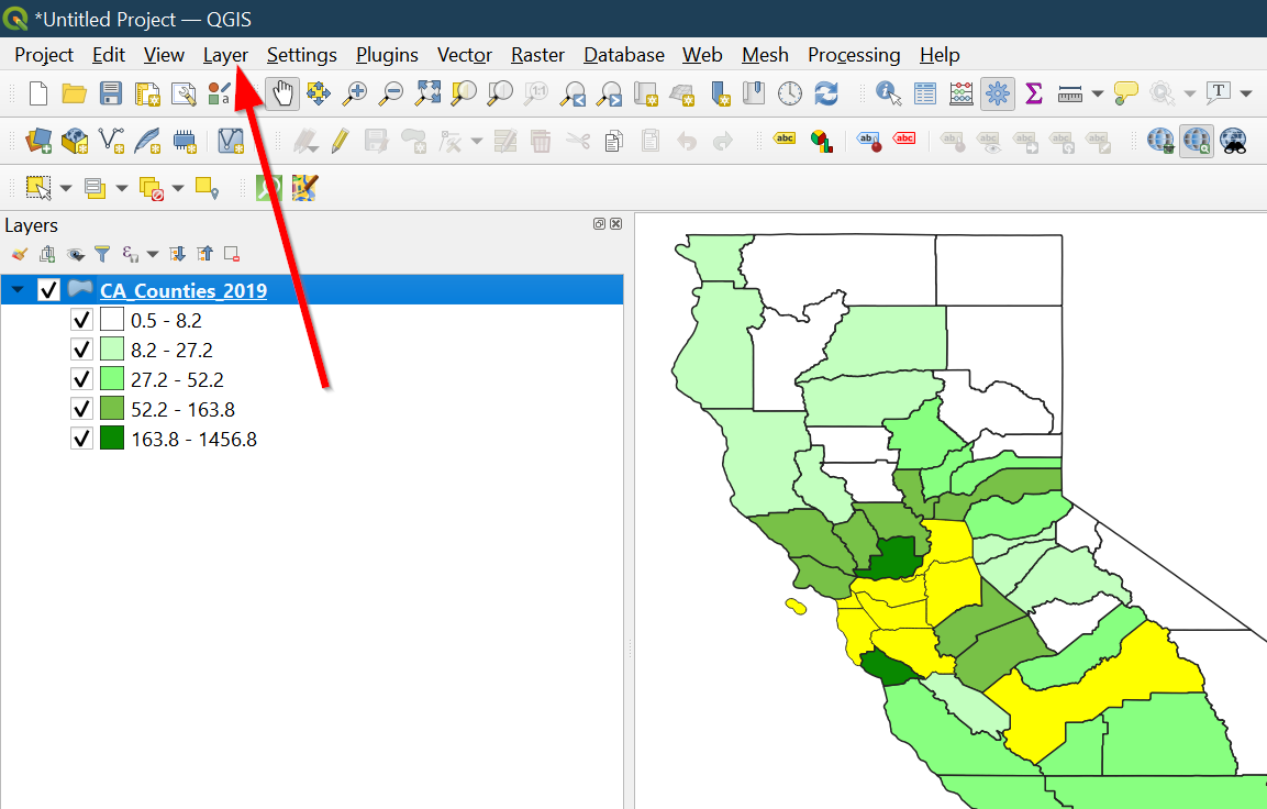
- You map should look like the following:
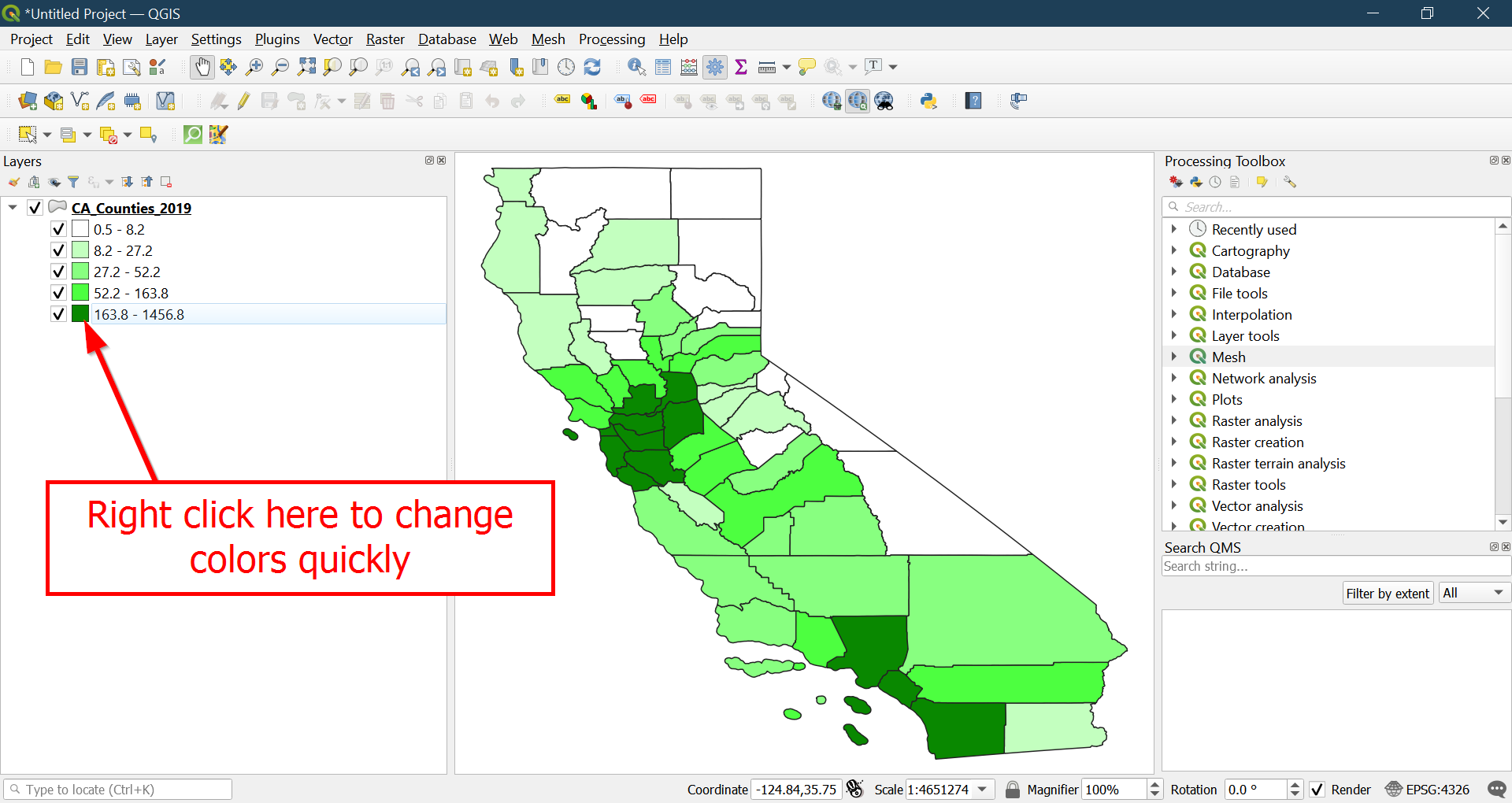
- Tip: You can quickly change any color by right clicking on the colored box to the left of any layer:
Filtering our fields
-
Let’s do some advanced filtering to see places where more than 100,000 Asians live.
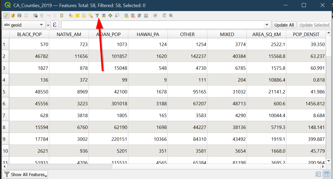
-
Start by opening our attribute table again:
- Right click on our layer
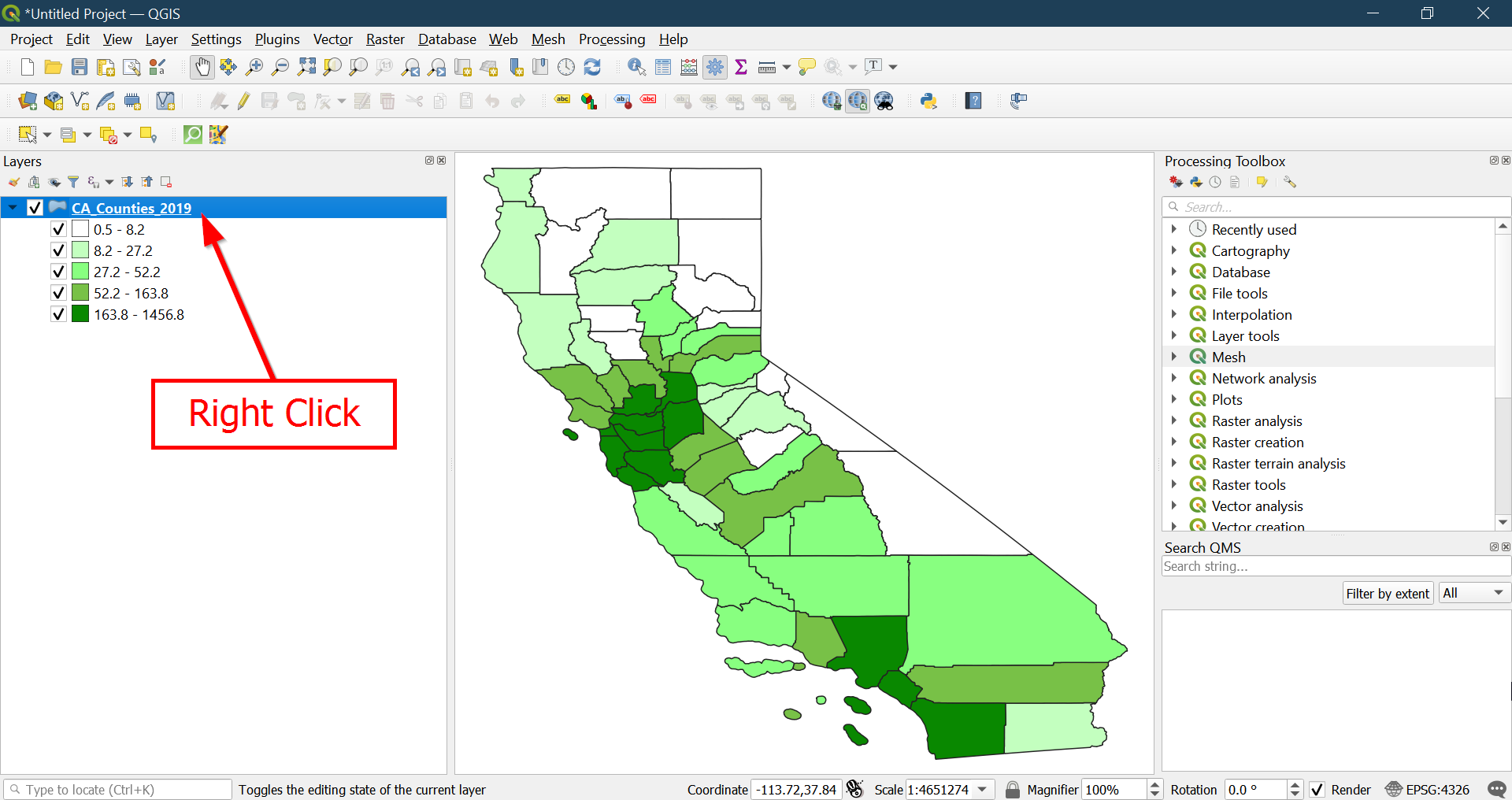
- Click
Open Attribute Table:
- Right click on our layer
- Click the
Filter selection form.
- We are finding places with
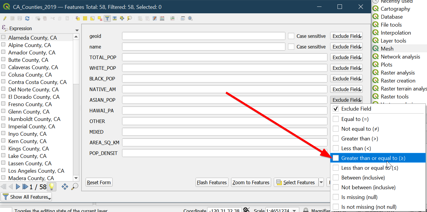
Asiansso locate theASIAN_POPfield:
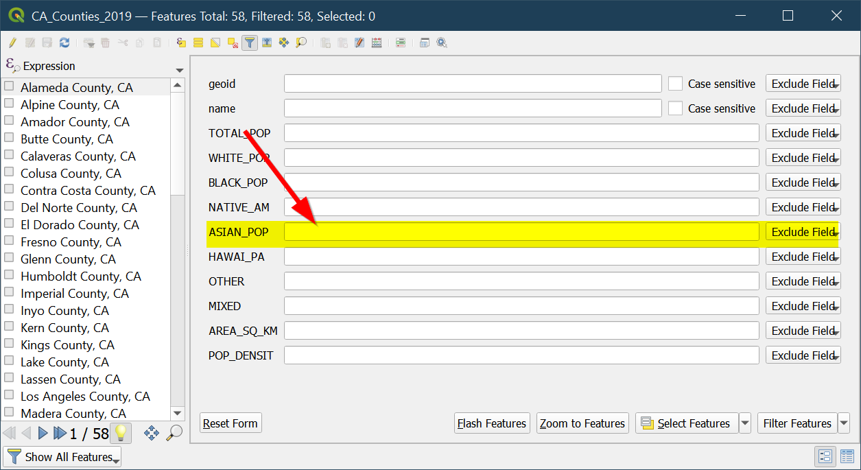
- Click the
Exclude fieldbutton to change it:
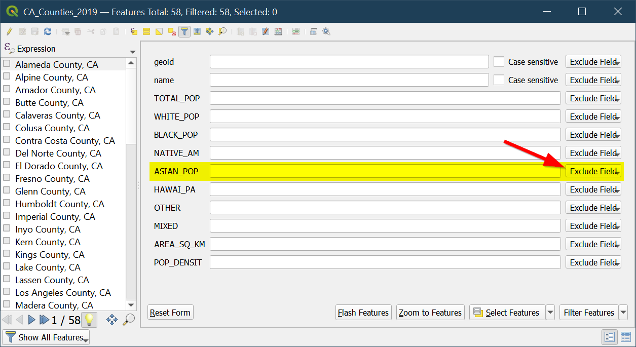
- We will make it
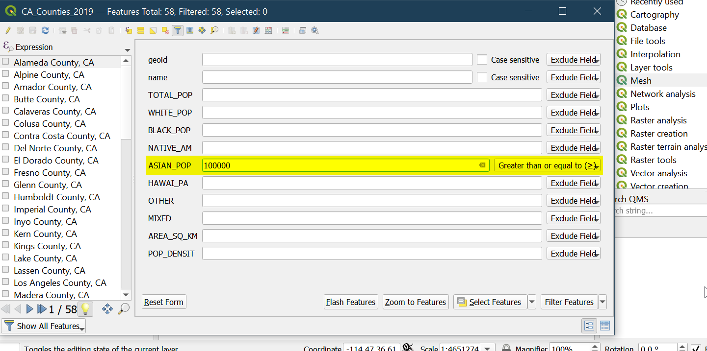
Greater than or Equal to:
- Then type in 100000:
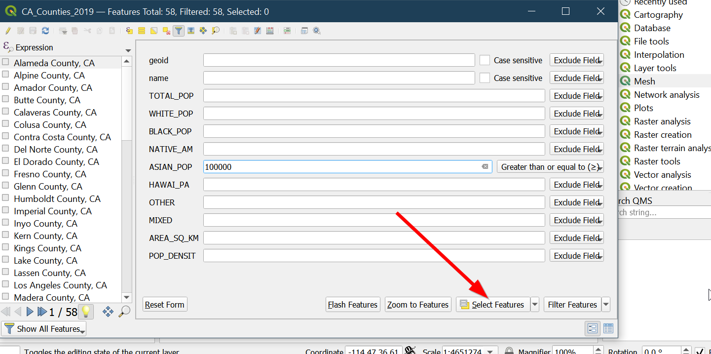
- Click on
Select Features
- Click the lower right icon to return to the table view:
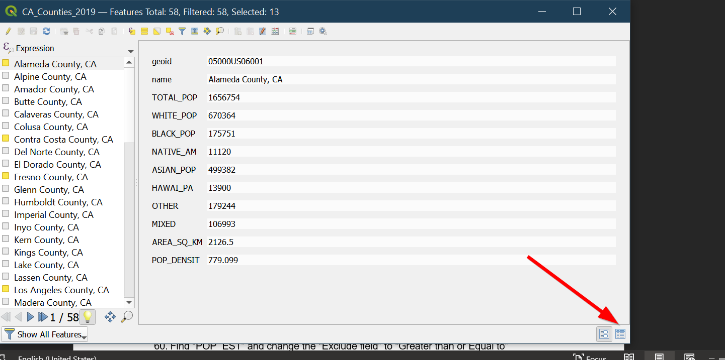
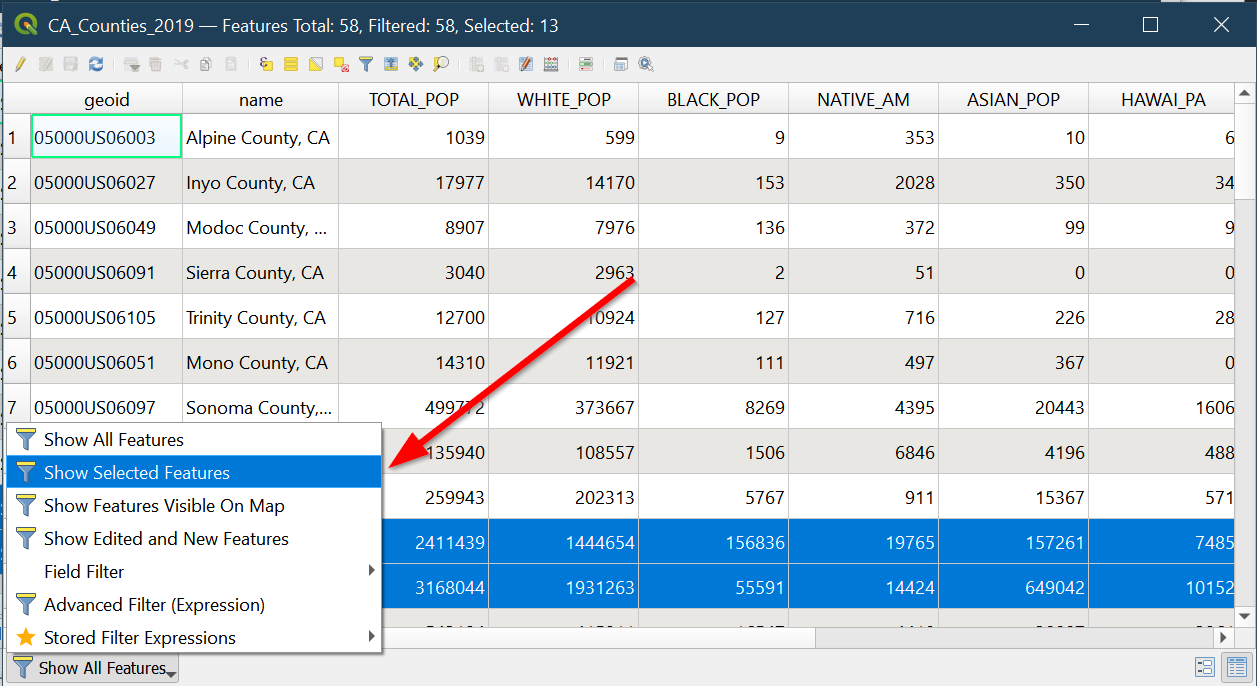
- You can view only selected features by clicking here:
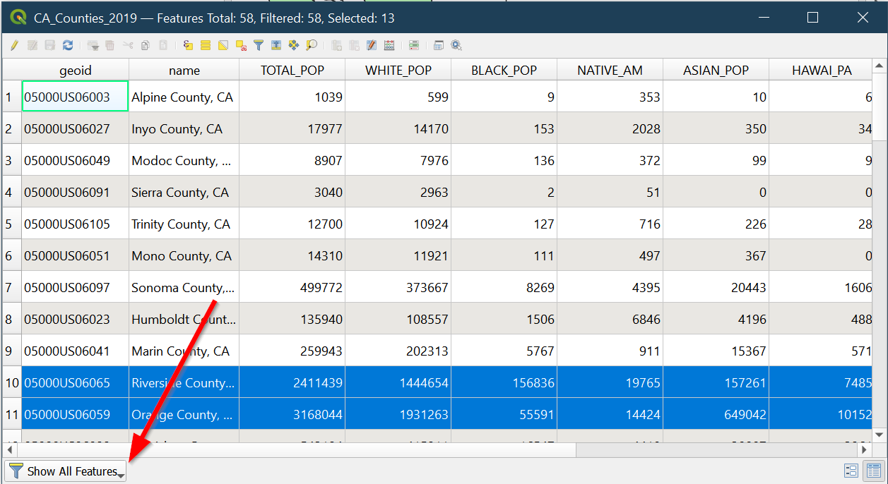
- Then choosing
Show Selected Features
- Close the table when done exploring by clicking the X:
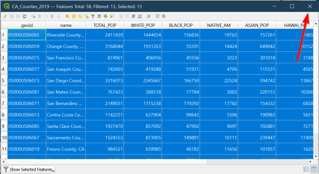
- Congrats! Now you have filtered some features.
Saving Our Map Layer for Web Mapping
- With everything still selected, right click on the layer:
-
Go to
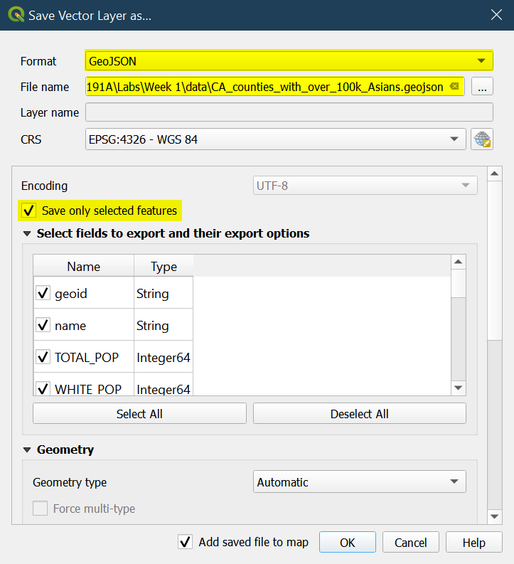
Exportand then chooseSave Selected Features As…: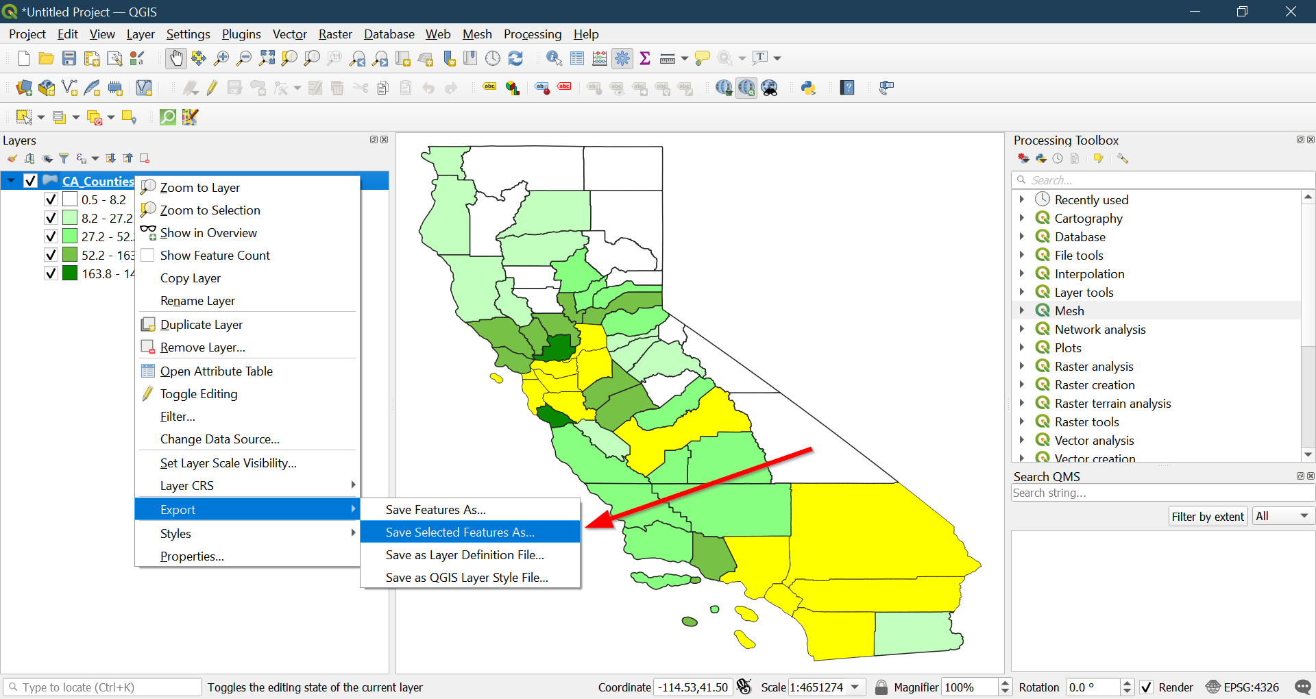
-
The ESRI shapefile is the default, but it is very hard to use in our web applications because it is a proprietary data format..
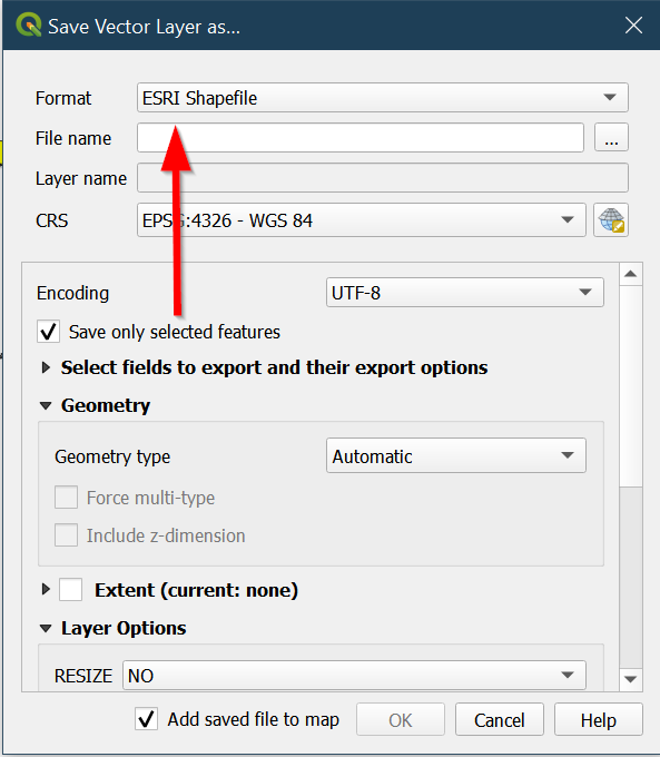
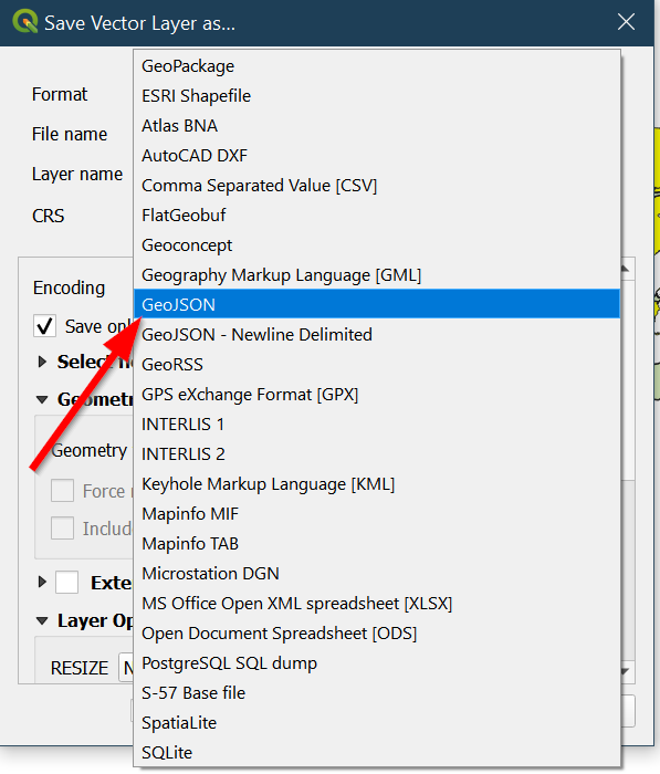
- The preferred spatial format online is a GeoJSON file:
- Click the
…next toFile Nameto find a nice new home for your GeoJSON file!
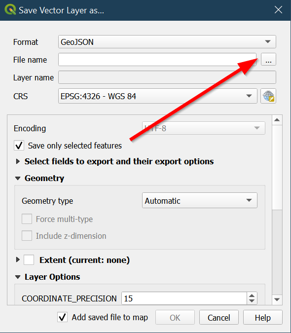
- Your final box should look like this:
-
Format: GeoJSON
-
File name: CA_counties_with_over_100k_Asians.geojson
- Congratulations! You have created your first
GeoJSONfile! We will revisit this file in next week’s lab, so keep it safe and sound!
Adding non-spatial data
- You can also add CSV files by clicking
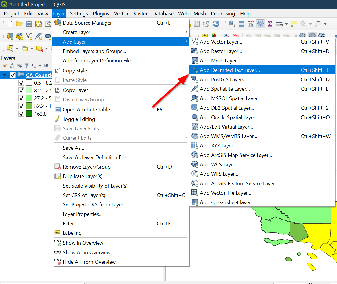
Layer
- Click on
Add LayerAdd Delimited Text Layer...
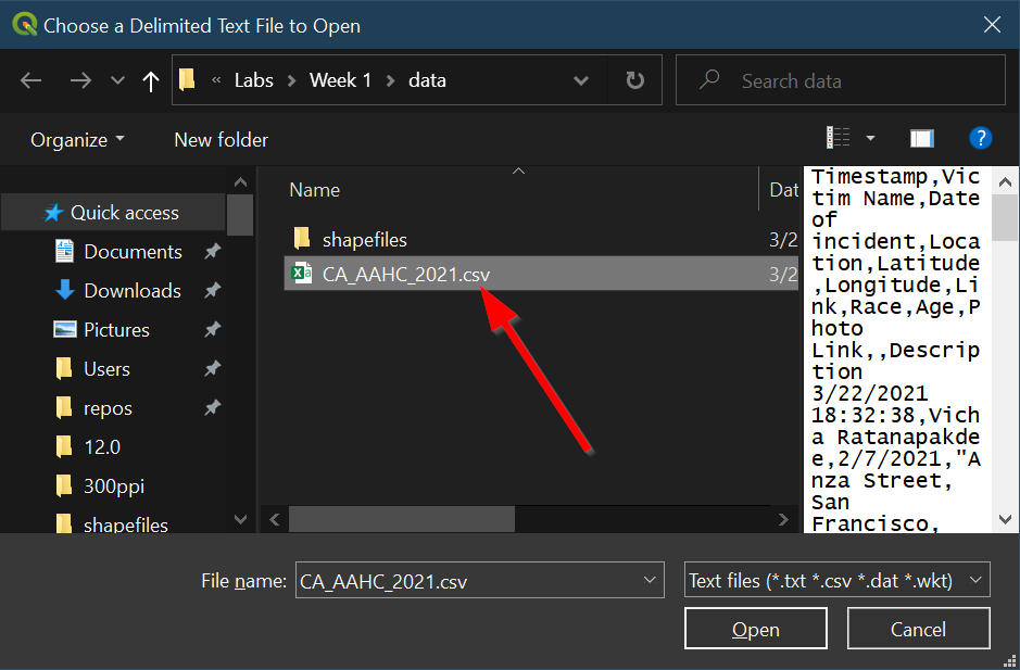
- To the far right of
File Name, click on the button with…:
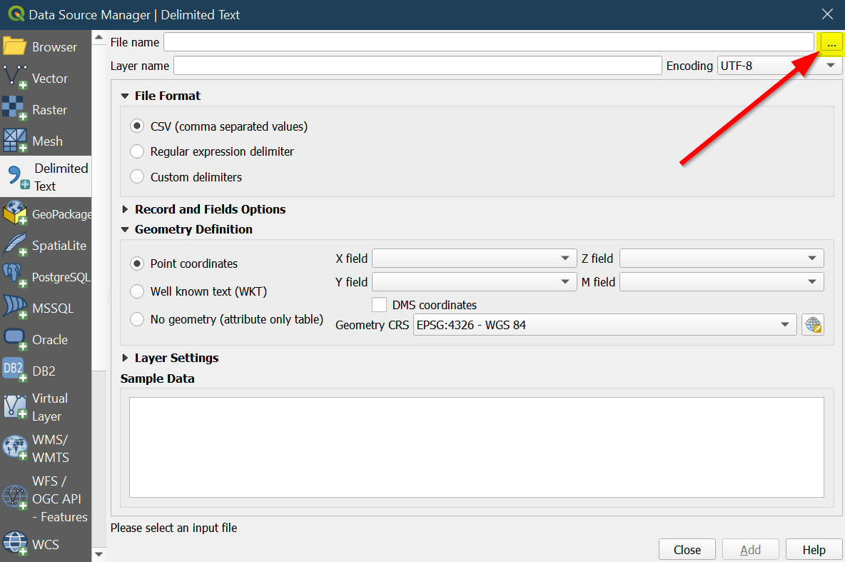
- Locate the file for California Asian American Hate Crimes,
CA_AAHC_2021.csv and select it and choose
Open:
- Check to make sure
Pointcoordinates and a coordinate reference system exists:
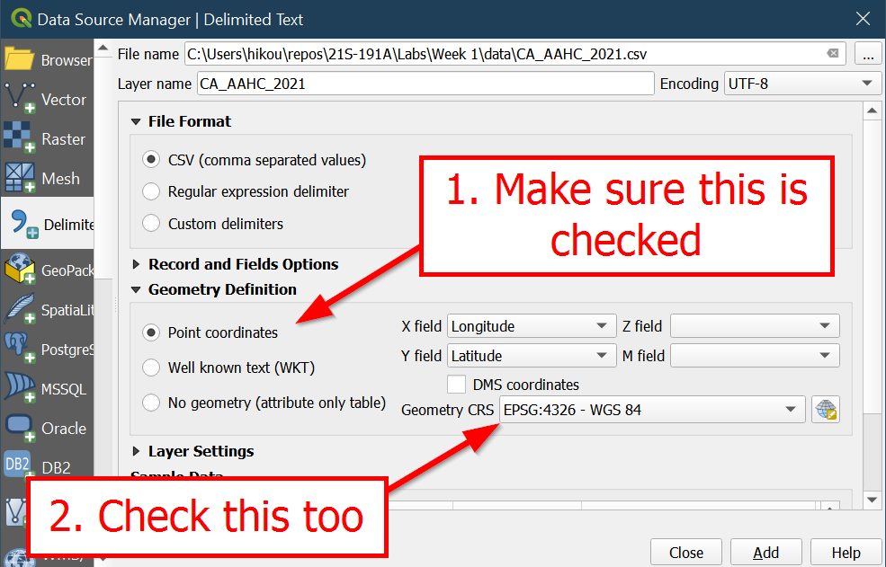
- Click
Addand thenClose:

- The data points should now show up:
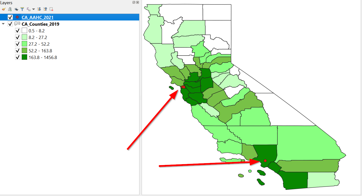
-
Note that you will not be able to edit CSV files, you will need to export them in a spatial data type format, such as shapefile or GeoJSON to do so.
-
Congratulations on finishing the spatial data management QGIS bootcamp.
Lab Questions
Please take some time to think about the following questions, they may be helpful when you are posting your Thinking Cap response for this week.
-
What changes did we make to the original data?
-
How can the choices we made in changing the data be problematic?